1) Graph only the data that are currently available in a data set that will continue to grow

2) Graph only the last so many entries in a data series

3) Graph only a part of a large data set (specify starting point and number of entries to show)

4) Graph only one column (year) out of a multi-column (year) data set

5) Use business terms to specify the starting point in 3)

6) Use a drop down box to specify the starting point in 3)

1) Graph only the data that are currently available from a data set that will continue to grow

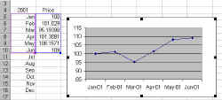
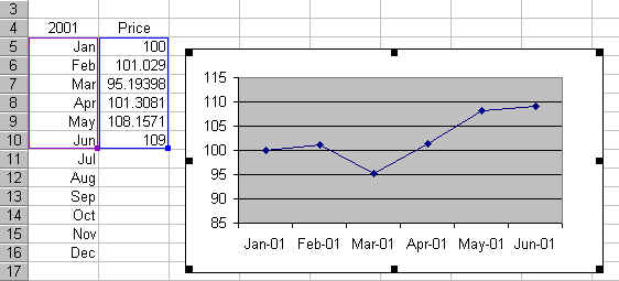
An example of the first would be a 'Year To Date' chart (see the example on the right).

Create the names

where 'Basic Range' is the name of the worksheet containing this example.  The '-1' in the definition of YValues adjusts for the cell containing the word 'Price' (cell B4).  Also, one must be careful and ensure that nothing else is entered in any cell in column B -- at least not without adjusting the formula above.

The next and final step is to create a chart with the formula
    =SERIES(,'Basic Range'!XValues,'Basic Range'!YValues,1)

2) Graph only the last so many entries in a data series

An example of this is a chart that displays only the last so-many elements of a large data collection.  The example on the right graphs the last 10 months of available data. This choice of 10 is controlled by the value in cell 'Show Last' (cell E1 in the example).

Create the names

where 'Last So Many' is the name of the worksheet containing this example.

Next, create a chart as in the above example.

3) Graph only a part of a large data set (specify starting point and number of entries to show)

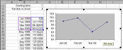
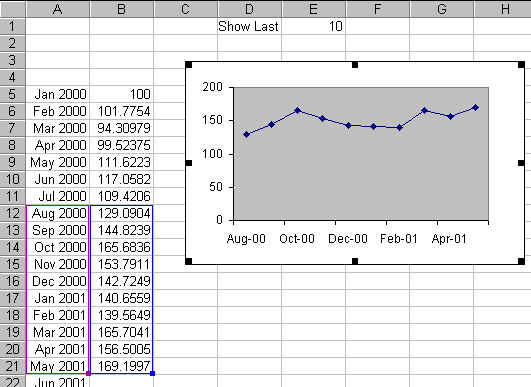
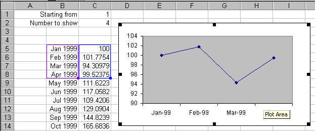
An example of this is a chart that extracts and displays only a portion of the information out of a large collection of data.  The example on the right graphs four months of data starting with month 1.  These choices are controlled by the values in the cells labeled 'Starting from' and 'Number to show' (cells C1 and C2, respectively, in the example).

Create the names

where 'Partial Range' is the name of the worksheet containing this example.

Next, create a chart as in the above example.

4) Graph only one column (year) out of a multi-column (year) data set

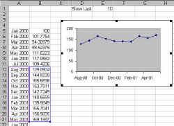
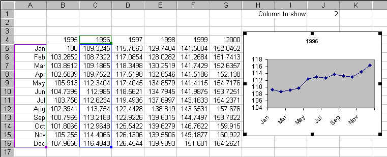
Another example would be a visual display of month-by-month data for just one year out of a 5 year collection of data.  The cell 'Which column' (cell J1 in the example) identifies the column that is currently shown in the graph.

Create three names (the third identifies the year currently shown in the graph):

where 'One column' is the name of the worksheet containing this example.

Create a chart with the formula:
=SERIES('One column'!WhichYear,'One column'!XValues,'One column'!YValues,1)

5) Use business terms to specify the starting point in 3)

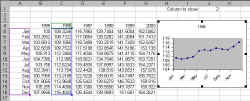
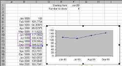
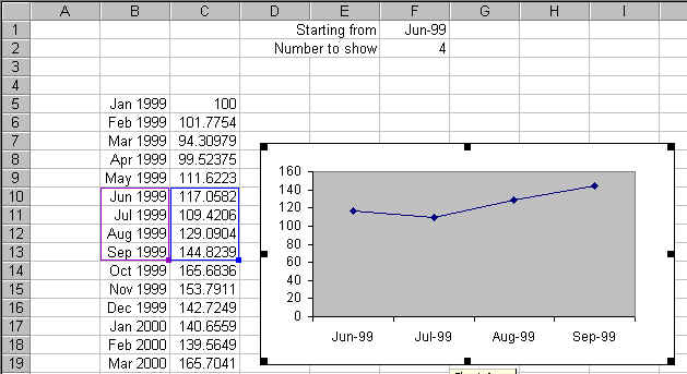
In 3) above, the starting point was specified relative to the first row containing the data.  From a business perspective it would be more natural to specify the starting point in the language of the business.  In this case, it would make more sense to specify the starting point as, say, 'June 1999.'

The OFFSET function still needs to know the starting row (the 2nd argument).  Consequently, the MATCH function provides a bridge between the starting date specified in F1 and the row number that Excel needs.  Also, to simplify the formulas a bit, the name XRange is used to define the range containing all the month values in column B.

where 'Business Partial Range' is the name of the worksheet.

A downside of this method is that someone can easily enter a value in F1 that has no match in the list of months.  The result will be cascading errors.

6) Use a drop down box to select the starting value in 3)

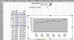
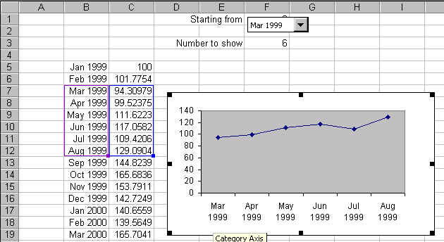
A further refinement is to use a drop-down box to get the starting row number.  In the event that one is asked to enter a date in the cell F1, it is possible the entry will be erroneous.  Using a drop down box eliminates the possibility.

The drop-down box puts the row number of the selected cell relative to the starting cell (as shown in the steps below).  Effectively, F1 now contains the same value as in 3) above, except that this is transparent to the user, who simply selects the month from the drop down list!

Since all the cell contents are the same as in 3), the same formulas and names apply.

where 'Partial Range Drop Down' is the name of the worksheet.  Also, note that XRange plays no direct role in the creation of the chart.  Its job is to simplify the creation of the drop down box.

Next, create the drop down box, make sure it covers cell F1.  Specify the Input Range as XRange, and the Cell Link as $F$1 (remember, it is easier and less error prone to click the cell with the mouse rather than type in the cell address)..