Names in Charts

You are on the Home/Excel/Tutorials/Dynamic Charts/Names in Charts page

After creating the named formulas, there are a few different ways to use them in a chart. For the examples in this page, we will use worksheet-level names as shown on the named formula page.

Creating a new chart

Updating an existing chart

Creating a new chart

Click on an empty cell that also has empty cells adjacent to it. Select the Chart Wizard button

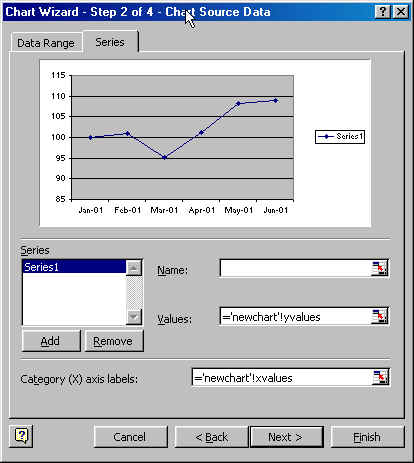
Select an appropriate chart type. For this example, use the Line Chart.

Click 'Next' and move to the Step 2. Click on the Series tab. Click the 'Add' button and fill in the names for the two series.

Note that in certain instances, Excel will replace the name provided with the current value of the named formula. If this happens, use the updating an existing chart method to correct the problem.

Updating an existing chart

There are two ways to update a series in a chart so that it now refers to a named formula.
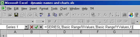
The most direct method is to update the series formula.
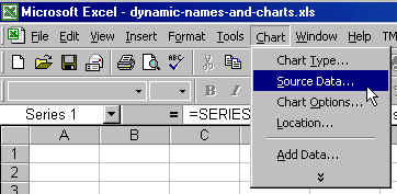
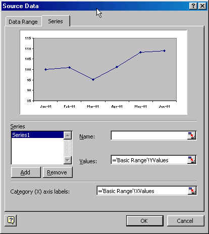
An alternative is to use the Chart... menu to update the Source Data... settings.

Updating the series formula directly

Select the series in the chart. Click in the formula bar and type in the names of the formulas as shown on the right.

Updating the Source Data... settings

Click on the series in the chart that is to be changed to the named formula. From the Chart menu select Source Data...

This brings up a dialog box that is very similar to the one in Step 2 of creating a new chart above. Of course, this time there is no need to add a series. Simply change the contents of the Values field and the Category (X) axis labels: field.