I came across a very reasonable request from someone who wanted to see which entries in a list matched those in the current cell (http://answers.microsoft.com/en-us/office/forum/office_2010-excel/event/49aa9987-3cf5-4007-9f08-df076ff0beba). While the original request dealt with names, I abstracted the problem into a set of numbers. Column A in Figure 1 is one list of numbers. Column C represents a list that we want to check against column A. Selecting a cell in column C should highlight all the matches in column A.
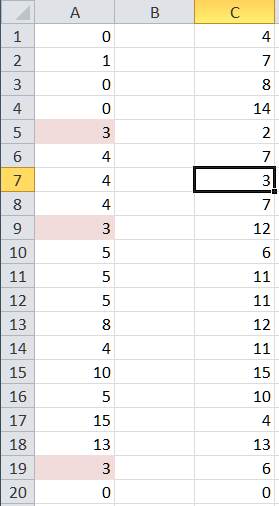
Figure 1
The intuitive approach would be to write the relevant code for the worksheet’s SelectionChange event procedure. However, in this context I have been, and remain, reluctant to do too much with code, primarily because it requires maintenance. In this case, any change to the ranges of interest, the insertion or deletion of columns, or a change in the desired format, such as the background color, would require code changes. In addition, the code can quickly get complicated. For example, one has to ‘undo’ the format when the selection changes, which means remembering the previous format for each of the cells in question.
An alternative approach uses an almost-never used variant of the Excel CELL function. The CELL function has two arguments. If the second argument, a cell reference, is missing, Excel substitutes the currently active cell.
So, select A1:A20, and create a conditional format. Choose the ‘Use a formula’ option specify the formula below and set the desired formatting. The formula specifies that if the active cell at the time of the recalculation is in column C, then return TRUE if the value of A1 matches that of the active cell. Otherwise, return FALSE.
Once the conditional format is set up, select a cell in column C and recalculate the worksheet (the shortcut is the F9 key).
The conditional format formula:
=IF(CELL("col")=COLUMN(C:C),A1=CELL("contents"),FALSE)
Figure 2
Finally, to avoid having to manually request a recalculation, put the code below in the worksheet’s code module:
Option Explicit
Private Sub Worksheet_SelectionChange(ByVal Target As Range)
Target.Calculate
End Sub

