This note documents a somewhat creative – and I suspect an unintended – way of using a slicer. A slicer is a control element introduced with Excel 2010. It is a large easy-to-use control to filter the results of one PivotTable or even multiple PivotTables. I like the UI look-and-feel of a Slicer and decided to explore it as a replacement for a data validation drop down list that has traditionally served as a selector.
So, instead of
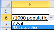
Figure 1
I wanted to use
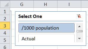
Figure 2
This also fit in very well with two other slicers I was already using to analyze the data.
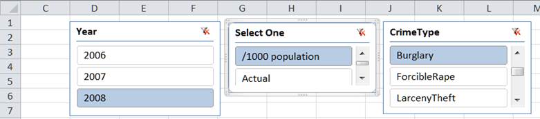
Figure 3
One common way to provide the consumer with a set of choices (in this case just two: actual data and per-capita data) is to use a data validation drop down list.
Select a cell in which the consumer will make the choice. Then, select Data tab | Data Tools group | Data Validation drop-down button. In the resulting dialog box, specify parameters as in Figure 4.
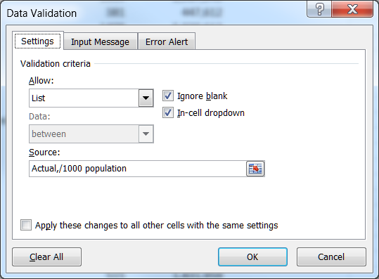
Figure 4
This yields a drop down list as in Figure 1. The advantage is that it fits nicely in a cell and works well with other data that the consumer may have to input.
Unfortunately, in this case, there are no other data for input. So this Data Validation list in a cell stands by itself – and its look-and-feel is rather incongruent with the Slicers available to control the dashboard.
A Slicer works with a PivotTable. So, create a dummy PivotTable that contains the 2 choices of interest (see Figure 5). Add a new worksheet to the workbook – I named this new worksheet SelectOne. In this new worksheet, create a list as in column D, where the 1st cell is the header. Then, create a PivotTable (Insert tab | Tables group | PivotTable dropdown) as in column F.
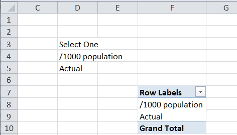
Figure 5
Next, add the slicer. Click in the pivot table and select Insert tab | Filter group | Slicer button. In the resulting dialog box, select the only available field.
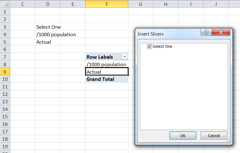
Figure 6
Now, select and cut the slicer object. Switch to the worksheet where the slicer is supposed to be and paste. I put it on the same worksheet as the other slicers (Figure 3).
Next, switch back to the worksheet and in the cell that should contain the choice, add a formula that refers to the 1st entry in the dummy PivotTable created above (Figure 7).
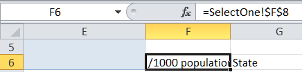
Figure 7
The only limitation that I can think of is that, unlike a data validation list, a slicer is not limited to just one choice. One can clear the filter and every item will be selected. Further, in cases where more than 2 choices exist, one can select multiple choices with the slicer. Of course, the formula (in the above example cell F6 in Figure 7) could be easily extended to ensure that only one item is selected. Do so by verifying that SelectOne!$F$9 equals “Grand Total”.

