Marty R on June 23, 2012:
Every time I come back to your site I find some gold nuggets -- 3 of them this afternoon! Special thanks for the conditional formatting coupled with active cell monitoring -- took me some work to apply it to an opportunity review tool we review weekly, but it will make our process go much more smoothly with the highlighting. And for the VABInStrRev function that will simplify a routine I created in the last 10 days managing a large number of files (wish I''d come to the site sooner! :) Thank You!
By default, when the user selects a cell, Excel highlights the row and column by changing the color of the associated row and column headers as in Figure 1.
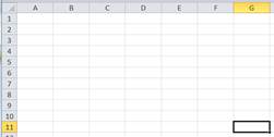
Figure 1
But, what if one wants a more visible indicator such as having the entire row and column highlighted as in Figure 2
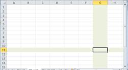
Figure 2
A variant of highlighting the entire row and column is to highlight the row to the left of the cell and the column above the cell as in Figure 3
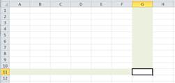
Figure 3
Yet another possibility is to use different colored borders for the row and the column as in Figure 4
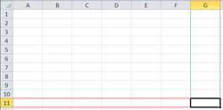
Figure 4
Another variant is to highlight a cell in a specific column and the same row as the selected cell. An example would be to highlight the ‘Account ID’ when one selects an ‘Amount Due’ entry as in Figure 5.
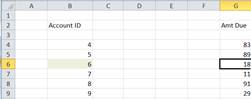
Figure 5
In this section, we will see how to accomplish the above exclusively through conditional formatting. The minimal VBA code required to make it work is the same single executable statement for all of the different highlighting options!
This same conditional formatting based approach works to highlight the rows and columns of a selection that spans multiple cells. While it does require more sophisticated code, this code too is a one-time development. The actual formatting is still completely contained in the conditional format.
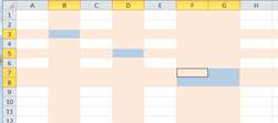
Figure 6
Download the Excel file with the code
In this section, we will look at various alternatives to focus attention on the selected cell. We start with the simplest approach.
Select cell A1 then select all the cells (click on the square at the intersection of the row and column headers).
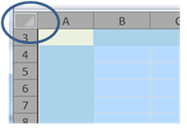
Figure 7
Next, select Conditional Formatting and create a condition based on a formula.
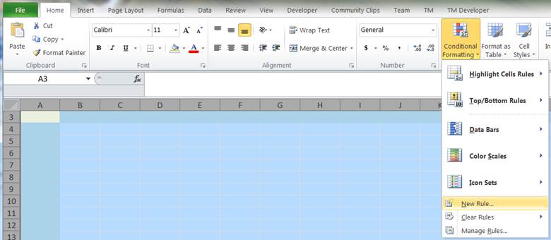
Figure 8
The formula should be =OR(CELL("col")=CELL("col",A1),CELL("row")=CELL("row",A1)). The formula returns TRUE if the cell is in the same column as the active cell or in the same row as the active cell. Also, add the desired format.
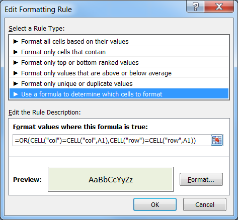
Figure 9
Now, select any cell and press F9 (recalculate). This will cause Excel to update the conditional formatting formula and the row and column of the selected cell will have a light green background as in Figure 2.
A very simple one-line VBA routine that will automate the recalculation is shown below. An additional benefit of this code is that it does not clear out the undo stack. Consequently, one can use undo even with this code active.
In the code module of the worksheet containing the conditional formatting:
Option Explicit
Private Sub Worksheet_SelectionChange(ByVal Target As Range)
Target.Calculate
End Sub
In this scenario, the programmatic support is the same as the above! There is no need to change the VBA code.
The only thing we need to do is change the conditional formatting formula. Use: =OR(AND(CELL("col")=CELL("col",A1),CELL("row")>CELL("row",A1)),AND(CELL("row")=CELL("row",A1),CELL("col")>CELL("col",A1))).
This will create a light green background to the left of and above the active cell as in Figure 3.
Once again, there is no need to change the code. All the work is through conditional formatting. Since we want a red border for the row and a green border for the column we have to use 2 separate conditional formats:
1) For the red row border, use the c.f. formula =AND(CELL("row")=CELL("row",A1),CELL("col")>CELL("col",A1)) and specify a format of red top and bottom borders.
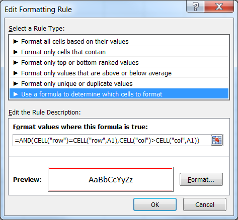
Figure 10
2) For the green column border, use the c.f. formula =AND(CELL("col")=CELL("col",A1),CELL("row")>CELL("row",A1)) and specify a format of a green left and right borders.
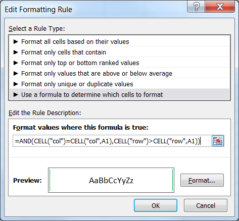
Figure 11
The combination of the two c.f.s will yield the result in Figure 4.
The technique shown in this tip has a range of applications other than just highlighting the row and column of the selected cell. One variant is to highlight a cell in a particular column and the same row as the selected cell as in Figure 5.
The same VBA module from above will work for this solution!
Suppose we want to highlight the cell in column B (starting with B4) whenever someone selects a cell in the same row in column G. To make this happen, select B4 then in the conditional formatting formula use =CELL("address")=CELL("address",$G4). Select an appropriate format and copy the format of B4 as far down as desired.
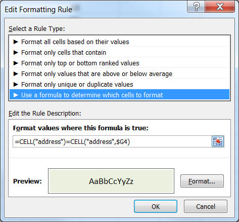
Figure 12
The use of CELL(“row”) or CELL(“column”) returns the row (or column) of the active cell only. So, even if one were to select multiple cells, the function will return a value for just the one cell. So, the above technique cannot be used to highlight multiple rows and columns (as in Figure 6).
We will develop a solution that is conceptually similar to the above in that the actual formatting will be through conditional formatting. So, changing the format will not require any update to the code. What we will do is create four named constants that will contain the first and last row and the first and last column of every selected area. Then, the c.f. formula will check if the cell falls within those row or column ranges. If it does, the c.f. format will apply. As an example, suppose we select C3 and E5:F6 and H8. Then, the named formulas created by the code will be:
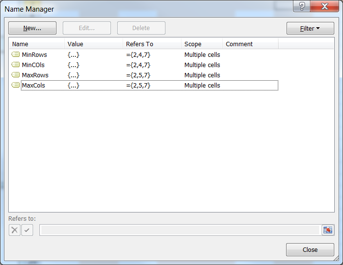
Figure 13
Now, the c.f. formula will check if the cell is between any of the above row pairs and between any of the column pairs. If so, the c.f. format will apply.
=OR(SUMPRODUCT((ROW(A1)>=MinRows)*(ROW(A1)<=MaxRows))>0,SUMPRODUCT((COLUMN(A1)>=MinCOls)*(COLUMN(A1)<=MaxCols))>0)
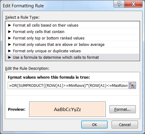
Figure 14
The code is not very complex. Also, remember this is a one time development. The formatting is done exclusively through the c.f. criteria.
The code below goes in the code module of the worksheet containing the above conditional formats.
Option Explicit
Private Sub Worksheet_SelectionChange(ByVal Target As Range)
Dim anArea As Range, MinRow As String, MaxRow As String, _
MinCol As String, MaxCol As String
For Each anArea In Target.Areas
With anArea
MinRow = MinRow & .Row & ","
MaxRow = MaxRow & (.Row + .Rows.Count - 1) & ","
MinCol = MinCol & .Column & ","
MaxCol = MaxCol & (.Column + .Columns.Count - 1) & ","
End With
Next anArea
With Target.Worksheet.Names
.Add "MinRows", "={" & Left(MinRow, Len(MinRow) - 1) & "}"
.Add "MaxRows", "={" & Left(MaxRow, Len(MaxRow) - 1) & "}"
.Add "MinCOls", "={" & Left(MinCol, Len(MinCol) - 1) & "}"
.Add "MaxCols", "={" & Left(MaxCol, Len(MaxCol) - 1) & "}"
End With
End Sub
A downside of updating named constants is that Excel will clear out the undo stack. So, we cannot use this technique and also support undo.
The conventional approach, which one can find via a search of the ‘Net, is to use VBA code to change the color of the cells in the corresponding row and column. This has four major downsides:
1) First, it overrides any formatting the consumer may have added to the affected rows and columns.
2) It requires undoing any previous highlighting, which requires some extra code to ensure that we do not leave any formatting in a saved workbook.
3) Any change to the desired format requires knowledge of VBA and modification of the code to implement the change.
4) Finally, it effectively disables Excel’s Undo capability.
To me these limitations constitute an extremely undesirable approach.

