Create a Dynamic (Self-Adjusting) Range

One of the most common issues that arise in Excel is that a range that contains data will eventually expand as more data are added or even contract as data are removed.  If we have a formula, or an Excel functionality (such as Data Validation or a PivotTable), or a chart, that refers to such a dynamic range, we must adjust the formula whenever the size of the range changes.  That is obviously impractical and is a major source of problems and errors in an Excel model.

Summary Results

For those who only want a solution without any explanation here are two options.

Suppose there is a range such as C2:C5 that contains data.  We want a create a reference to this range in such a way that as new data are added in C6, C7, etc., all the references to the range adjust to include the new data.

The first option is to use a Table in Excel 2007 or Excel 2010 (called a List in Excel 2002 and Excel 2003).

Now, any existing reference to the cells in the table – such as =SUM(C2:C5) – will expand to include any new data added to the table.  To learn how to create a table see the section Create a Table (called a List prior to Excel 2003).

If we create a reference to the data after we create the table, Excel will refer to the cells as Table{n}[{ColumnName}], e.g., Table1[Score]

The second option is to use a named formula that returns a range reference, e.g.,

aRng     =OFFSET(Sheet1!$C$2,0,0,COUNTA(Sheet1!$C:$C)-1,1)

After creating this named formula, often called a dynamic range, use it to refer to the current range.  So, instead of =SUM(C2:C5) use =SUM(aRng).  This named formula relies on the data being contiguous.  For more in this subject and for an alternative that works with missing data see the section Using a Named Formula.

The rest of this tip describes the problem and the solutions in more detail.

The problem description

Three typical examples showing a formula, a conditional format, and a Excel functionality (Data Validation in this case) are below

The SUM function is a pretty straightforward application:

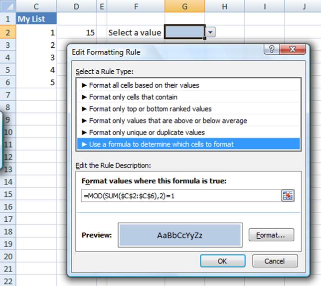
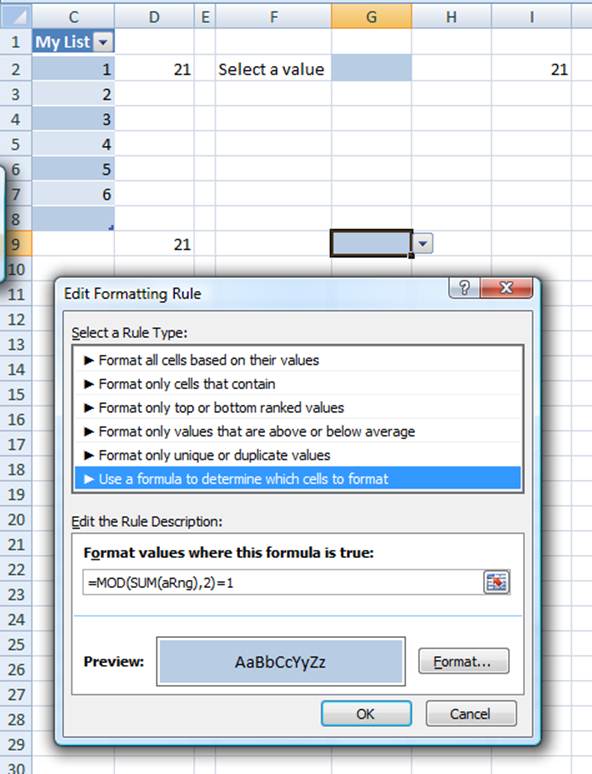
The conditional format, applied to cell G2 causes the background to be blue if the sum of the cells in the specified range is odd:

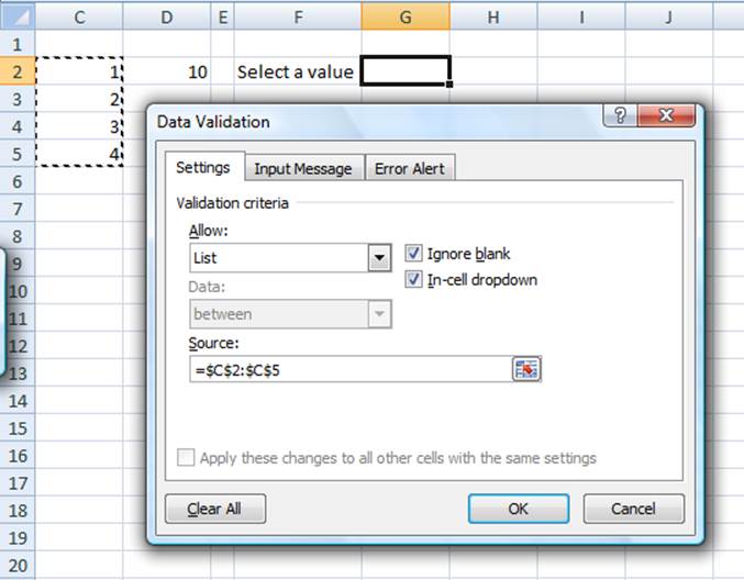
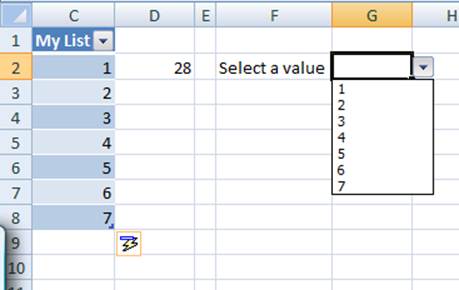
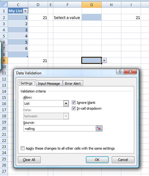
In the third example, the data validation allows a choice of items from the cells in the specified range.

The problem with each of the above is that as we add new data in C6, C7, etc., we will have to keep track of all the cells and functionality that we will have to update.  So, if we were to add all integers up to 7 (going down to cell C8), we would have to know which cells and dialog boxes we must update to reflect the new data.

Clearly, that is an impractical solution.  Below, we look at two possible ways to address this problem.  As is often the case, there are multiple approaches possible, each with its pros and cons.  The discussion below will address the limitations of each method.

Create a Table (called a List prior to Excel 2003)

Newer versions of Excel (starting I believe with Excel 2002) support the Table feature (called a List prior to Excel 2007) in which Excel itself updates references to the table range as the size and contents of the table change.  However, this capability was not fully implemented in 2003 in the sense that a conditional format failed to update itself when more data were added to a List.  The advantage of this method is that it is easy to implement and Excel will do all of the bookkeeping required to make it work.  It does have some limitations as discussed later in this section.

To create a Table in Excel 2007 or Excel 2010, use Insert | Table and in the resulting dialog box specify the current range of the table.

In 2003, use Data | List > Create List… and the same dialog box as above will appear.

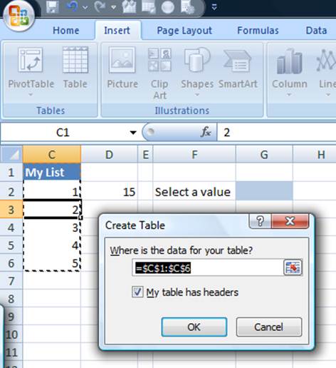
The result, in 2007 (it looks similar in 2003):

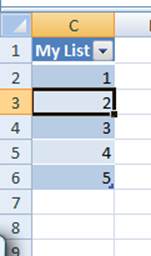
Now, when new data are added to the list the various locations where the range appears will be updated automatically.

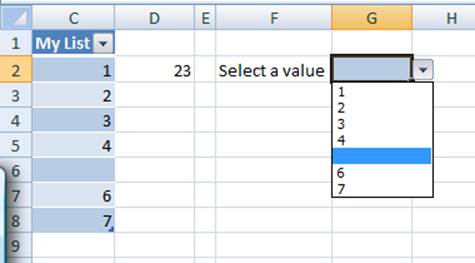
Note that the formula in D2 now totals 28, the Data Validation drop down shows the expanded list and the c.f no longer shows a blue pattern.

Excel will correctly handle missing data.  So, if the 5 in the table above is deleted, the various formulas and capabilities will update correctly.

While Excel 2007 updated the conditional formatting formula correctly, the same does not apply to Excel 2003 in which the c.f. formula will not be updated – one can verify this quite easily.

Another instance where Excel will not update a formula – and this should not be a surprise – is if when the range is specified as an argument to the INDIRECT function as in =SUM(INDIRECT("C2:C5")).

 Yet another place where it does not work is in a reference from another workbook.  Actually, this works when both workbooks are initially open. However, after they are closed and reopened, the link is apparently severed.

A final and important limitation is that the reference will always be to the entire column in the table (or list).  We cannot have a reference to just a portion of the table, such as the last N rows.  This capability can be important for those instances where one wants a moving total or moving average or one wants to plot only the last so-many values of a data set.

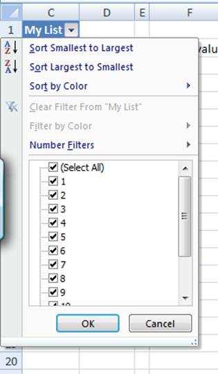
An additional benefit of the Excel 2007 table approach is that Excel supports additional capabilities for the table itself.  One can explore these features, which include sorting and filtering, by clicking the drop down button.  The Excel 2003 List features similar though fewer capabilities.

Using a Named Formula

An approach that has worked since at least Excel 97 is to use a named formula that correctly identifies the range of interest.  The use of this formula results in dynamic range, which adjusts itself as data are added or subtracted from the range.  In addition to working with many more versions of Excel than the previous method, this technique also supports the ability to refer to only a subset of the data.  This makes it possible to create formulas to calculate the moving average.  It is possible to define this subset in several different ways.  One can even create a resulting set that repeats the data – a technique that can yield a “closed” graph!

To identify all the cells in a contiguous range, use the OFFSET function with the COUNTA function as in

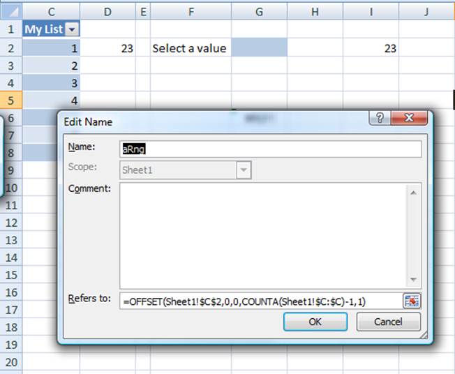
The COUNTA function returns the number of cells in column C that contain data.  We subtract 1 to exclude the column header.  Then, the OFFSET calculates a range starting with C2 (offset by zero rows and zero columns) with a height given by the number of cells containing data and a width of 1 column.

Now, use the name aRng in place of a range reference.  So, =SUM(aRng), or, for a data validation source use =aRng.  Similarly, use with the formula of a chart series, or in a conditional formatting formula would all be valid uses of aRng.

For example, in the conditional formatting for G9 we would use

To use the named range in the Data Validation specification we would replace, as above, the reference to the range by the name of the formula as in:

In all these instances as we add data to C8, C9, etc., Excel will correctly update the various results and functionalities.

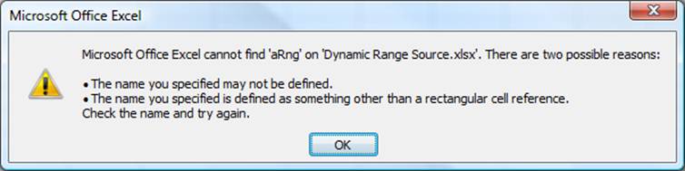
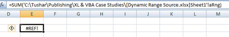
One limitation of this approach is that it does not work if the name is defined in a workbook that is currently closed.  One must open that workbook before Excel will update calculate the correct result.  While the source workbook is closed, Excel will display an error dialog box and the cell will calculate as a #REF! error as shown below.

Another limitation of this named formula approach using the OFFSET and COUNTA functions is that it does not work if the range includes missing data.  One can adapt the Named Formula approach to such instances by using a long-present bug in the Excel MATCH function[1].  While I don’t like this approach because it exploits a bug, I suspect Microsoft will never correct this bug because so many have exploited it for so long that the behavior has become the norm rather than the exception.

When the last argument of the MATCH function is 1 the data are expected to be in ascending order.  But, even if they are not, Excel assumes they are.  So, a search for the largest possible number 9.9999999999999999E307 will always locate the last number – though, frankly, I don’t know what will happen if the number is actually present in the table.  There are limitations to this technique in that if the data contain text, one must match REPT(CHAR(255),255) rather than 9.9999999999999999E307.

To use this approach, define a new name, aRng3 as

aRng3

=OFFSET(Sheet1!$C$2,0,0,MATCH(9.99999999999999E+307,Sheet1!$C:$C,1)-ROW(Sheet1!$C$2)+1,1)

After defining this name, use it in place of aRng above.