Each of the following solutions takes very little work -- and each is implemented strictly in Excel. In addition, the coding techniques demonstrate some VBA programming methodologies that are themselves quite non-traditional.
For a variety of reasons, one expects a solution designed in Excel to conform closely to the defaults provided by Excel. That often results in worksheet based solutions that rely on a tabular grid or a VBA solution with a userform with some number of buttons and various controls in shades of grey. However, as this tutorial demonstrates, it is possible to create solutions that are close to the consumer's expectation of the interface for a particular device (a telephone, in this case).
The problem at hand is to develop a mechanism to convert phone "numbers" that contain letters into pure numbers. Yes, the task is seemingly trivial and can be accomplished with Excel formulas, albeit non-trivial ones. At the same time, this seemed an ideal candidate to illustrate some less-traditional user interfaces coupled with equally non-mainstream programming techniques.
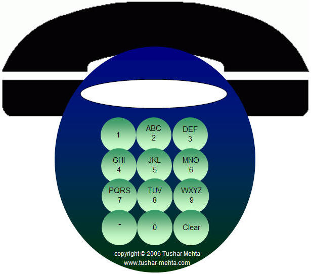
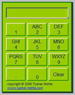
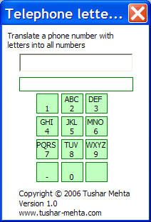
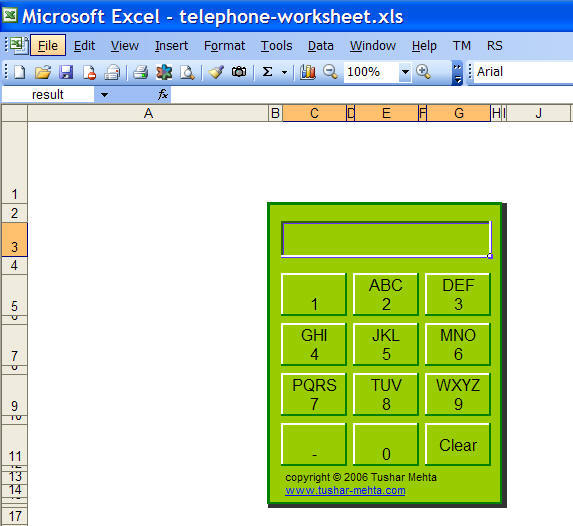
The user interfaces of the three solutions discussed below are shown in Figure 1. The first UI uses shapes and an image. The second is simply Excel cells formatted to create the desired effect. The last should be easily recognizable as a userform, albeit with all the grey removed.
 |
 |
 |
All the solutions use VBA code. However, as we will see the coding itself is as non-traditional as it is simple.
1 The zip file contains three files, each of which contains one of the above solutions. Each file contains VBA macros and it is up to you to decide if you want to open the file or not.
The final effect is the combination of the Oval shape from the Drawing toolbar. with an image of the handset. The latter was either from the Microsoft Clipart collection or from a search of Google images.
To create a circle, click the Oval shape in the toolbar, hold down the SHIFT button and drag to draw.
To align objects, select them, then from the Drawing toolbar select Draw | Align or Distribute > and the appropriate alignment option.
To add text, select the object, right-click and select the Add Text item. Set the font and font size appropriately and for the object set the Margins as desired (double-click the object, then in the resulting dialog box, click the Margins tab, and set the various margins).
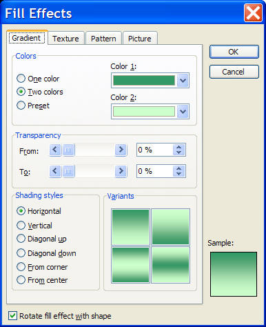
| The fill used for each shape was a dual color effect. To accomplish this select the object, then select Edit | Format Autoshape... (or simply double-click the object). In the resulting dialog box, select the Colors and Lines tab. From the Color drop-down select Fill Effects... |
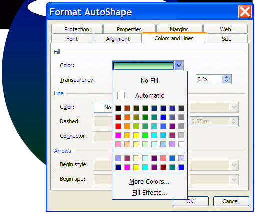 |
| In the Fill Effects dialog box, select the Two Colors option and set the colors as desired. |
 |
Once one circle is completed, duplicate it to create the others, the easiest way being to copy it, paste 11 times, and make the necessary changes to each.
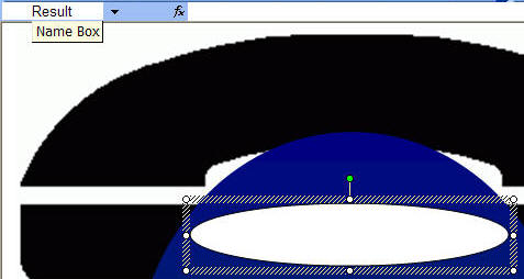
| Name the oval that will contain the result
(it's the only white object) as Result. To
do this, select the object, then type the name in the Name Box
and press ENTER.
|
 |
Next, add the macros. How many lines of code do you think we need to add? How about 2 lines? Well, other than the subroutine declarations. It turns out we need a few more since once we protect the worksheet, the code cannot update the Results shape without unprotecting the sheet first. In a standard module, add the following:
Option Explicit
Sub clearResult()
    With ActiveSheet
    .Unprotect
    .Shapes("Result").TextFrame.Characters.Text = ""
    .Protect
        End With
    End Sub
Sub aDigit(aDig As String)
    With ActiveSheet
    .Unprotect
    With .Shapes("Result").TextFrame.Characters
    .Text = .Text & aDig
        End With
    .Protect
        End With
    End Sub
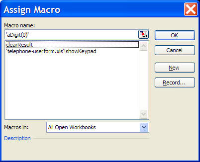
| To assign a macro to each circle,
right click the object, then select
Assign Macro... In there use
the not-well-documented method of assigning a macro with a
argument value. For example, the digit 0 assignment would
be as shown to the right. Note the use of single quotes
around the entry.
|
 |
| To assign the minus sign, the assignment
statement is slightly different in that it requires the minus
sign to be enclosed in double quotes. For more on this technique see
|
 |
Put the final touches to the display. Delete all the sheets in the workbook other than the one with the telephone pad design. To remove most of the typical Excel interface elements, select Tools | Options... Then, from the View tab, uncheck the options for:
Gridlines,
Row & column headers,
Horizontal scroll bar,
Vertical scroll bar, and
Sheet tabs.
Accomplishing the effect of raised buttons and a sunken result space requires the combination of three separate steps.
First, leave alternate rows and columns blank. Reduce their respective widths or heights. For those rows and columns that will become 'buttons' make them reasonably large. Re-adjust these once again to get the best effect after completing the other steps.
Second, the raised effect requires the following: Use a light shade for the patterns for all the cells in the region. For each cell that will be a button, draw a white border on the top and left edges, and a dark border for the right and bottom edges. [For a sunken effect as in the Result field, reverse the white-dark selections. However, for a reason that will become clear in a bit, we will have to reformat the border colors for the result field.]
Third, for the finishing touch, enclose the overall region that will be the telephone dialpad with a thick border. Create the shadow effect by making the next right column and bottom row very narrow and filling the cells with a black pattern.
To enter the letters and the number on a separate line, use the ALT+ENTER combination. Remember to use ALT+ENTER even for those cells that contain only a single character (the 1, the zero, and the dash sign). This is important since the VBA code relies on the presence of the character corresponding to ALT+ENTER.
Next, widen column A and row 1 so that the telephone pad appears more towards the center of the monitor.
Create the space that will contain the result with the following: First, merge cells B3:G3. Select them, the right-click, select Format Cells... and from the Alignment tab check the option Merge Cells. Name this merged cell as Sheet1!Result -- assuming the worksheet is named Sheet1.
The result cell borders must be formatted slightly differently than the other cells. This is because when Excel selects a cell it "reverses" the border color after accounting for the color of the cell's interior. So, when selected, a white border will become pink. Since we will always have the result cell as the selected cell, the white should be the result after Excel applies it reverse the border color algorithm. Since white becomes pink, start with a pink border and Excel will reverse it to white!
Also, name the cell that contains the word "Clear" as CLR.
The final formatting touches are similar to the previous option. Delete all the sheets in the workbook other than the one with the telephone pad design. Remove most of the typical Excel interface elements: Select Tools | Options... Then, from the View tab, uncheck the options for:
Gridlines,
Row & column headers,
Horizontal scroll bar,
Vertical scroll bar, and
Sheet tabs.
Next, the code.
We will use the worksheet's SelectionChange event procedure to detect which cell the user clicked. The code will use the value of the cell to figure out what digit to add to the result cell. In addition, it will always leave the result cell as the selected cell. This is important since the SelectionChange event is not triggered if the user selects an already-selected cell. A discussion of how this code is non-mainstream is left to a separate section since it would not quite fit in with the UI emphasis here and it would make this section incredibly long. So, here's the code without a detailed explanation.
Insert class module and name it clsWKS. In it, insert the code below:
Option Explicit
Dim WithEvents WKS As Worksheet
Property Set aWS(uWS As Worksheet)
    Set WKS = uWS
    End Property
Private Sub WKS_SelectionChange(ByVal Target As Range)
    Dim aName As Name
    If Target.Cells.Count > 1 Then GoTo ErrXIT
    On Error Resume Next
    Set aName = Target.Name
    On Error GoTo 0
    If aName Is Nothing Then
    ElseIf InStr(1, aName.Name, "CLR") > 0 Then
        WKS.Range("Result").Value = ""
        GoTo NormalXIT
        End If
    Dim vbNewLineLoc As Integer
    vbNewLineLoc = InStr(1, Target.Value, Chr(10))
    If vbNewLineLoc < 1 Then GoTo ErrXIT
    WKS.Range("result").Value = WKS.Range("result") & _
        Mid(Target.Value, vbNewLineLoc + Len(Chr(10)), 1)
    GoTo NormalXIT
ErrXIT:
    Beep
    GoTo NormalXIT
NormalXIT:
    On Error Resume Next
    Application.EnableEvents = False
    WKS.Range("result").Select
    Application.EnableEvents = True
    End Sub
In the ThisWorkbook module, insert the code:
Option Explicit
Dim WSManager As clsWKS
Private Sub Workbook_Open()
    Set WSManager = New clsWKS
    Set WSManager.aWS = ActiveWorkbook.Sheets(1)
    End Sub
Private Sub resetHandler()
    Set WSManager = Nothing
    End Sub
The resetHandler code is needed if one wants to make any change to the worksheet design. Run it before making worksheet changes.
This section discusses the userform design and presents the code without any discussion. As above, the code discussion is deferred to elsewhere. See xxx for an explanation of how it all works. One note though. The entire implementation is through objects. Each task is performed by the object best suited to that task (well, actually, by the code in the class module that defines the object).
To test the final solution, from Excel run the showKeypad macro (use ALT+F8 to display the Macros dialog box, then double click the showKeypad entry). Typically, I would use a menu item or a toolbar but implementing that interface would needlessly distract from the focus of this section.
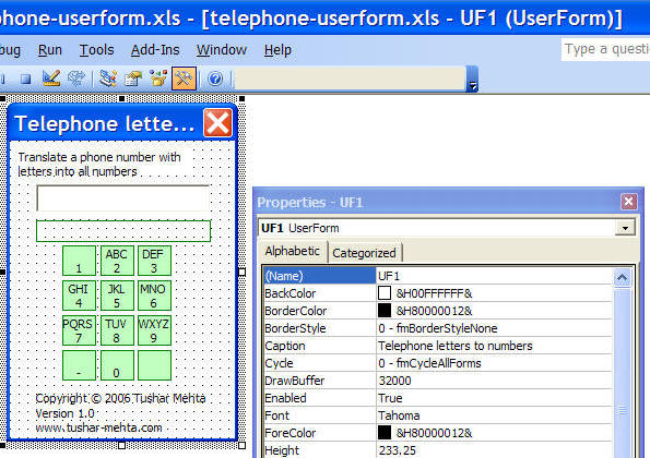
Create a default userform. Reshape it so that it is longer than wider. Change the background color to white. To do so, select the userform, then click F4 to bring up the Properties pane. In there set the BackColor to white. Also change the name to UF1 and the caption to something more appropriate than Userform1.
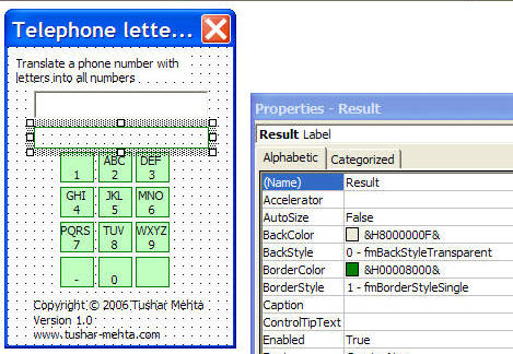
Each of the controls is a label with the exception of the field in which the user can enter a phone number, which is a Textbox.
For the labels that are not green, click each and from the Properties pane set the BackStyle to transparent. Name the label that will contain the result as Result.
In creating the green labels, it may be more efficient to create one label, format it as desired, then copy-and-paste to make additional labels.
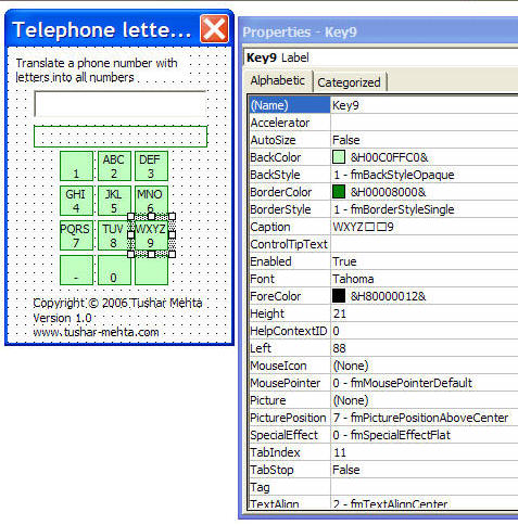
For those labels with a green background, set the BackColor to an appropriate light color. In those labels, to separate the letters on one row from the number on the 2nd row, use the CTRL+ENTER combination. Format the height and width to get the desired effect.
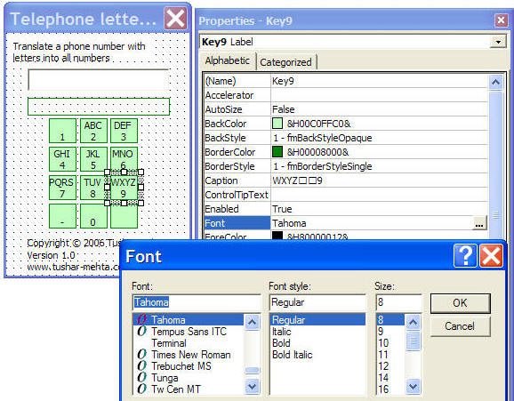
Format the font for each label by clicking the Font entry in the Properties pane, then clicking the ...button that shows up on the right to call up the Format Font dialog box.
Name each label as Key1, Key2, etc. Name the label with the hyphen as KeyMinus and the label with the empty caption as Clear. Optionally, use a caption for that key that reads Clear or something along those lines.
The code required to make the userform work is presented here without discussion. See xxx for an explanation of how it all works. The only point worth noting here is that the implementation is exclusively through objects. The only piece that isn't is the code needed to show the userform. And, that too would be part of an object if I'd created a menu for this solution. But, the code to create a menu and handle the user selections would have needlessly distracted from the focus of the solution. The result is the one-liner standard module.
The code in the UF1 userform's module:
Option Explicit
Dim allLabels As Collection, _
    Translator As clsTranslator
Private Sub Clear_Click()
    Me.UserText.Text = ""
    End Sub
Private Sub UserForm_Initialize()
    Dim aCtrl As MSForms.Control, LabelWithEvents As clsLabel
    Set Translator = New clsTranslator
    Set allLabels = New Collection
    For Each aCtrl In Me.Controls
    If TypeOf aCtrl Is MSForms.Label And Left(aCtrl.Name, 3) = "Key" Then
        Set LabelWithEvents = New clsLabel
        Set LabelWithEvents.aLabel = aCtrl
        allLabels.Add LabelWithEvents, LabelWithEvents.aLabel.Name
        End If
        Next aCtrl
    End Sub
Private Sub UserText_Change()
    Dim i As Integer, Rslt As String
    For i = 1 To Len(Me.UserText.Text)
        Rslt = Rslt & Translator.Translate(Mid(Me.UserText.Text, i, 1))
        Next i
    Me.Result.Caption = Rslt
    End Sub
Public Sub insertText(aText As String)
    Dim Temp As String, Rslt As String
    With Me.UserText
    Temp = .Text
    Rslt = Left(Temp, .SelStart) & aText
    If .SelStart = 0 And .SelLength = 0 Then
    Else
        Rslt = Rslt & Right(Temp, .TextLength - (.SelStart + .SelLength))
        End If
    .Text = Rslt
        End With
    End Sub
The code in the standard module:
Option Explicit
Sub showKeypad()
    UF1.Show
    End Sub
The code in the class module named clsLabel
Option Explicit
Dim WithEvents aLbl As MSForms.Label
Property Get aLabel() As MSForms.Label
    Set aLabel = aLbl
    End Property
Property Set aLabel(uLabel As MSForms.Label)
    Set aLbl = uLabel
    End Property
Private Sub aLbl_Click()
    Dim vbNewLineLoc As Integer
    vbNewLineLoc = InStr(1, aLabel.Caption, vbNewLine)
    If vbNewLineLoc < 1 Then
        UF1.insertText aLabel.Caption
    Else
        UF1.insertText _
            Mid(aLabel.Caption, vbNewLineLoc + Len(vbNewLine), 1)
        End If
    End Sub
and finally, the code in the class module named clsTranslator
Option Explicit
Dim Letters() As String, Numbers() As String
Function Translate(aVal As String)
    On Error Resume Next
    Dim Rslt
    With Application.WorksheetFunction
    Rslt = .Match(aVal, Letters, 0)
    If Err.Number <> 0 Then
        Translate = aVal
    Else
        Translate = .Index(Numbers, Rslt)
        End If
        End With
    End Function
Private Sub Class_Initialize()
    Letters = Split("A,B,C,D,E,F,G,H,I,J,K,L,M,N,O,P,Q,R,S,T,U,V,W,X,Y,Z", ",")
    Numbers = Split("2,2,2,3,3,3,4,4,4,5,5,5,6,6,6,7,7,7,7,8,8,8,9,9,9,9", ",")
    End Sub

