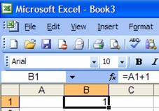
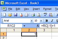
Introduction

The traditional way to enter a formula in a spreadsheet has been to refer to cells by their default cell references.  In Excel, this typically means either the A1 or the R1C1 convention.  For example, if in cell B1, we want a formula that adds 1 to the value in cell A1, we would use =A1+1 or its R1C1 equivalent of =RC[-1]+1

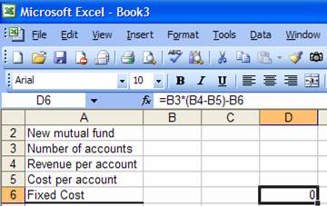
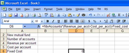
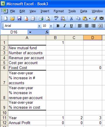
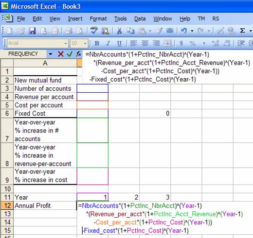
This is typically more than adequate for simple formulas.  Even the formula below is relatively easy to understand.  It calculates the annual profit of a new mutual fund taking into account the unit-profit, the number of accounts, and the fixed operating cost.

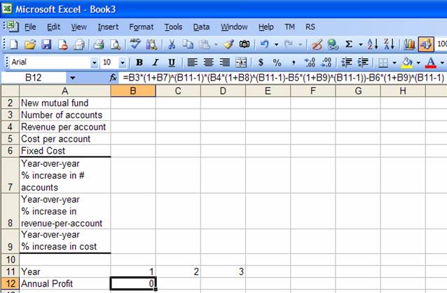
But, how about trying to understand the formula below?  It calculates the annual profit as above but now it factors in the expected annual increases in each of the components.

In this chapter we look at how to make formulas easier to understand.  We will do that in two ways.  The first uses names to replace cell references and the other formats a formula to bring out its structure and hence make it easier to read.

Named Cells – the default absolute address

Instead of using the default cell reference, one can always name a cell.  The quick way to do this is to use the name box, which is at the extreme left of the formula bar.

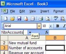
To name cell B3 as NbrAccounts, select the cell, then click in the Name Box, type the name and press the Enter key.

Figure  1 – Naming cell B3: snapshot taken just before pressing the Enter key

A slightly more complicated way but also one that includes more advanced options is to use the Define Name… dialog box (accessed via Insert | Name > Define…)

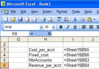
Name the cells B4, B5, and B6 as Revenue_per_acct, Cost_per_acct, and Fixed_Cost respectively.

List the names and use names instead of cell references

To see the list of all names, select a cell in an otherwise empty range of the worksheet, then select Insert | Name > Paste…  In the resulting dialog box, select Paste List.

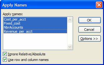
Once a cell is named, one can use the name instead of the cell reference.  The easiest way to replace cell references in existing formulas is to have Excel to do the needful.  Select a single cell, then Insert | Name > Apply…  In the resulting dialog box, select all the names and click OK.

In every cell in the worksheet that contains a formula, Excel will replace the cell reference corresponding to each name with the name itself.

Now, isn’t that a lot easier to understand?  Essentially, it makes the formula self-documented.

To use a name in a new formula, just create the formula as usual by clicking on each cell.  Whenever a clicked cell has a name, Excel will use it instead of the reference.  Alternatively, one can always simply type the name.

Worksheet and Workbook names

Here are two questions to consider:  If we name a cell on one worksheet, can we refer to that cell on another worksheet using its name?  On the flip side, can we assign the same name to different cells in different worksheets?  The answer to both questions is “yes.”

To refer to a cell on another worksheet that has already been named, one need do nothing different.  While entering the formula, simply click on the cell of interest.  Excel will automatically use the name rather than the cell reference.

To understand how we can assign the same name to cells on different sheets, we need to understand the difference between a workbook-level name and a worksheet-level name.  When we create a name as above, it is known as a workbook-level name and can essentially be used in any worksheet in the workbook.  However, it is also possible to create a worksheet-level name.  To do this precede the name with the worksheet’s name as in

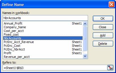
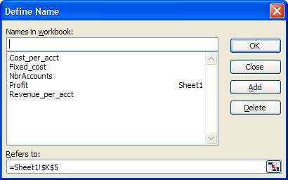
If the worksheet name contains anything other than letters and numbers, it must be enclosed in single quotes.  Typically, I add the single quotes every time.  That way I don’t have to worry about whether or not the quotes are required.

How does one know if a name is a worksheet-level name or a workbook-level name?  The difference shows up in the Name dialog box (Insert | Name > Create…)  This dialog box lists all workbook-level names and all names associated with the current worksheet.  In addition, each worksheet-level name shows the worksheet name in the column on the right.

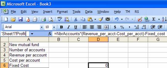
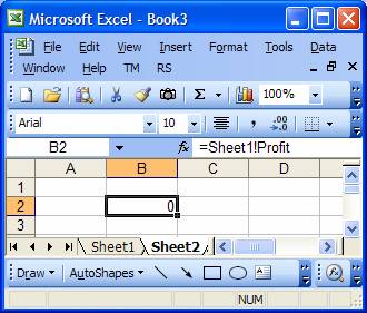
Once we understand the concept of a workbook and a worksheet name, it should be evident that one can create the same name at the worksheet-level in different worksheets.  So, in Sheet1, one might name cell C5 as Sheet1!Profit and in Sheet2 one might name cell D12 as Sheet2!Profit.

To use a worksheet name, once again, one need do nothing different.  Just click on the cell while building a formula and Excel will automatically use the sheet-level name as in

Named Cells – the power of a relative address

So far each name refers to a specific cell using what is known as an absolute address.  Essentially, no matter what cell is the current cell, a formula that refers to that name refers to a specific cell.  For example, no matter where we enter the formula =NbrAccounts, we are always referring to cell B3 on sheet Sheet1.

Yet, as we saw in xxx, in an Excel formula we can use absolute or relative addressing (and even mixed absolute-relative addressing).  The same capability applies to named cells.  Suppose we want to track the profit for each of three years as in:

Once we name cells B7:B9 appropriately, the formula in B12 is

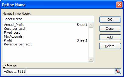
=NbrAccounts*(1+PctInc_NbrAcct)^(B$11-1)*(Revenue_per_acct*(1+PctInc_Acct_Revenue)^(B$11-1)-Cost_per_acct*(1+PctInc_Cost)^(B$11-1))-Fixed_cost*(1+PctInc_Cost)^(B$11-1)

We can also replace the mixed reference to the year (B$11) with a name.  First, select any cell in column B.  Then, create a name using Insert | Name > Define…  In the resulting dialog box, make sure the reference to the cell uses mixed-addressing as below.

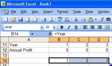
Excel remembers that we had selected a cell in column B when creating the name Year, which had a relative reference to column B.  Hence, wherever we use the name Year, Excel will always interpret it to refer to the cell in the current-column row-11.

We can test this quite easily.  In some cell, say B14, enter the formula =Year.  Copy B14 to C14:D14.  The cells should show the values 1, 2, and 3 respectively.

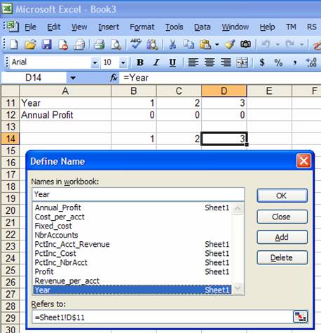
Another way to see how Excel interprets the name is to select a cell in some column other than B, bring up the Define Name dialog box (Insert | Name > Define…) , and select the name Year.  The ‘Refers to’ field will refer to the cell in row 11 of the current column.

We can now modify the formula for the Annual Profit (B12) so that it reads:

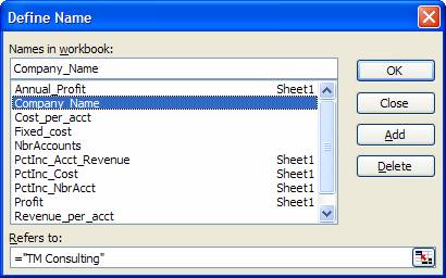
=NbrAccounts*(1+PctInc_NbrAcct)^(Year-1)*(Revenue_per_acct*(1+PctInc_Acct_Revenue)^(Year-1)-Cost_per_acct*(1+PctInc_Cost)^(Year-1))-Fixed_cost*(1+PctInc_Cost)^(Year-1)

Named constants

In addition to referring to a particular range, a name can also be just a constant.  For example, if one plans to use the name of the company in several cells in different worksheets, it might make sense to create a named constant such as

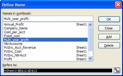
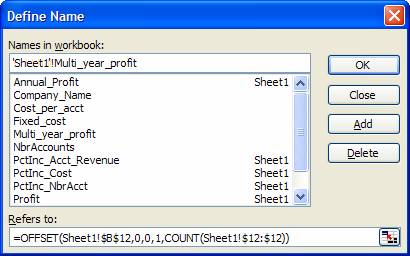
While this is a perfectly legitimate use of Excel names, I am not a big fan of this approach.  To me it would make a lot more sense to put all such constants in a worksheet and then name those cells making the design of the workbook is a lot more transparent and easier to understand.

Named multi-cell range

So far, the names we have used referred to a single cell.  That is not a requirement.  One can name a range of cells using the same method used for a single cell.  Hence, select a range of cells and use the Define Name dialog box (Insert | Name > Define…) to name the range.  Alternatively, type in the name (optionally, making it a worksheet level name) in the Name Select the three cells corresponding to the 3 annual profits and enter a name for this range.  In the example below, we name the range ‘Sheet1’!Multi_year_Profit.

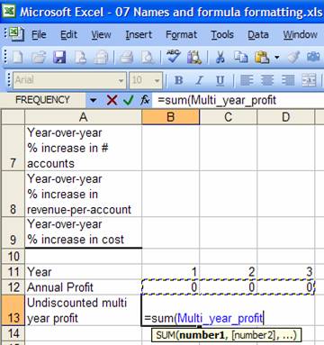
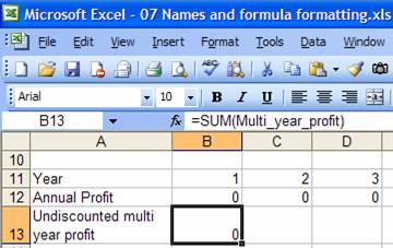
Once we name a range, we can use the name in place of the range reference just as in the case of a named single cell.  For example, to calculate the total of the undiscounted cash flows, we would use =SUM(Multi_year_profit).  In fact, Excel automatically recognizes the name and uses it as soon as we select the 3 cell range (see below).

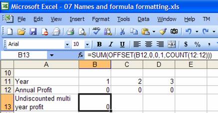
Named Formula

Suppose we wanted to extend the above analysis to include an additional year, i.e., Year 4.  All of the names above, with the exception of the last one (Multi_year_profit) would work just fine as we extend the model by adding an extra column (column E).

Unfortunately, the name Multi_year_profit, which refers to a specific range encompassing multiple cells, would continue to refer to B12:D12 and would not automatically extend to include E12.

As we will see soon, named formulas play a critical role in creating solutions that automatically adapt to changing data set.  This is particularly true in creating a chart that adapts itself to additional rows (or columns) of data or when using an array formula.  In the case of the former, a named formula becomes necessary because one cannot specify a formula as a chart series but one can specify a name that resolves to a formula.  In the case of the latter, it is because one cannot refer to an entire row or an entire column in an array formula.

Of course, none of the above limitations applies to our example.  Nonetheless, it makes sense to introduce the concept of named formulas in this chapter.  [In our specific case, instead of having Multi_year_profit refer to the range B12:D12, we could easily have it refer to the entire row 12:12.  This simple change would lead to a correct solution for any number of years.]  But, let us look at how to create a formula that refers to a range B12:{x}12 where {x} can be D or E or, for an analysis of an even longer duration, some other column further to the right.

A particularly useful function is OFFSET.  This function returns a reference to a range of cells based on five arguments (some of which are optional): reference, rows, columns, height, and width.  Reference can be any range that will serve as the starting base reference.  Rows is a number indicating the number of rows we should offset from the base reference we get the actual start address.  Columns is a number indicating the number of columns to offset from the base to get the actual start address.  Height indicates how many rows to include in the final range reference and width indicates the number of columns to include in the final range reference.  For a more detailed explanation of this very powerful capability, see xxxyyy.  For our purposes, we want to create a dynamic range reference 1 row high and several columns wide starting with cell B12.  How many columns wide?  We use the COUNT() function to figure that out.  COUNT returns a count of the cells that contain a number.  So, the formula =OFFSET(B12, 0, 0, 1, COUNT(12:12)) returns a reference to the range starting with B12 and including all the cells in row 12 that contain a number.  Now, we can wrap that with a SUM function to get the desired result.

Of course, the next step is to improve the readability of the worksheet with a named formula.  Suppose we were to replace the range reference in the name Multi_year_profit with the OFFSET formula.  We would get:

And, the newly defined name would be used as

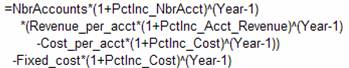
Formatting a formula

By default, Excel creates a formula as a stream of characters with no formatting to distinguish what operators and functions are nested within others.  Essentially, we cannot see the structure of the formula.  For an example of such a formula see the formula for the ‘Annual profit’:

=NbrAccounts*(1+PctInc_NbrAcct)^(Year-1)*(Revenue_per_acct*(1+PctInc_Rev_per_acct)^(Year-1)-Cost_per_acct*(1+PctInc_Cost)^(Year-1))-FixedCost*(1+PctInc_Cost)^(Year-1)

However, it is quite easy to bring out the structure in the formula.  One can force a new line within a formula with ALT+ENTER and one can also introduce white space by simply use the space bar.  The result of doing so with the annual profit cell is:

Note that the color in the formula is something that Excel itself adds whenever one is editing a formula.  The color of each item also matches the border that Excel temporarily adds to the corresponding cell.

An add-in that lists all names in a comprehensive list

Summary

By naming cells and by formatting formulas to bring out their structure, this chapter showed how to dramatically improve the readability and maintainability of Excel formulas.  The example used in the chapter converted the formula  into .

We also laid the groundwork for more advanced analysis by introducing the subject of named constants, named multi-cell ranges and named formulas.