Excel supports two different ways to filter data that are in tabular format. Autofilter is a built-in capability driven via the user interface. As sophisticated as Autofilter has become in recent versions of Excel, no pre-defined setup can possibly cater to all the different questions that the consumer may want answered. These require a custom filter and Advanced Filter provides that capability. It is a data-driven mechanism that uses Excel formulas to extract specific information from the original data. For those who may have heard of SQL but have never been motivated to learn it, you can now leverage some of the power of SQL without learning a single word of SQL!
The primary version of Excel for this document is Excel 2010 but the techniques should work with older versions of Excel (Excel 2007 and Excel 2003) with some changes to the terminology (e.g., an Excel 2010 Table is an Excel 2003 List).
Filter and sort are complementary but otherwise totally different capabilities. A filter uses a consumer defined criteria to show a subset of the original data. An example might be to show all customers whose orders remain unshipped. On the other hand, to sort data means to keep the entire original data set intact but to organize it in a way convenient to the consumer. An example of sort might be to organize the data so that the customer names are in alphabetic order or so that the orders are shown in descending sequence based on the ordered quantity.
For those who are unfamiliar with AutoFilter (or would like a refresher), search Bing (or Google) or visit http://office.microsoft.com/en-us/excel-help/filter-data-in-a-range-or-table-HP010073941.aspx
The layout of this document is as follows: 1) Introduction to the data set used in the examples, 2) Introduction to the Advanced Filter dialog box, 3) Filter using column headers, 4) Filter using Excel formulas, 5) Extract unique data, 6) Work with dynamic source data, and 7) Create a filter in a different worksheet or workbook.
Filters: Autofilter and Advanced filter
Filter in-place or Copy to another location
Specify filter criteria with column names
Example 1: Specify a simple single condition
Example 2: Specify 2 AND conditions
Example 3: Specify 2 AND conditons on the same column.
Example 4: List only specific columns in the output
Example 5: Specify an OR condition
Example 7: Leading text search
Example 8: Text search for an exact value
Example 9: Text search with wildcard
Example 10: Text search with 2 wildcards
Example 11: Working with dates I – Simple date condition
Example 12: Working with Dates II – Two AND date conditions
Example 13: Working with dates III – Empty dates
Specify filter criteria with a formula
Example 14: A simple formula as a filter criteria.
Example 15: A calculated field as a condition – I
Example 16: Use a formula to combine multiple conditions
Example 17: Use a formula with multiple Excel functions
Example 18: A calculated field as a condition – II
Example 19: Consolidate data from related rows
Example 20: Compare the row ‘value’ relative to the overall data set
Advanced Filter criteria must be a regular formula and not an array formula
Example 21: Advanced Filter criteria with a workaround to an array formula
Example 22: Unique records with a single output column
Example 23: Unique records with multiple output columns
Example 24: Unique records that meet a condition
Working with dynamic source data
Example 25: Consolidate data from related rows
Working with source data in a separate worksheet or a separate workbook
Before diving into the different ways Excel provides of filtering data we will look at the sample dataset that we will use for the rest of the chapter. The data set is a modified version of a table from the Northwind database that Microsoft has used for several years in its examples. The modifications to the data specifically make the already fairly rich dataset more useful in understanding Excel’s filter capabilities. Also, the modifications replace the long string “Northwind Traders” that starts every product name with the shorter “NT.” A sample of the first few rows of data together with all the column headers is in Figure 1.
The table provides information about the status of each item in each order placed by customers. When a customer places an order, it is given a unique Order ID. Each product is uniquely identified by Product. If an order includes multiple products, there is one row in the table for each combination of Product & Order ID. For each order-product combination, the table tracks the order date (Order Date), the product ship date (Shipped Date), which will be empty if the product is not yet shipped, the customer name (Customer), the quantity ordered (Quantity), and the unit price (Unit Price).
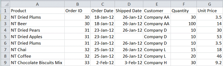
Figure 1
We will explore a range of management questions that we can answer with Advanced Filter in support of business operations.
Advanced Filter provides many features for data-based filtering that are not available in AutoFilter. Because Advanced Filter works with the data and not the formatting, the color-related capabilities of Autofilter are outside the scope of an advanced filter. At the same time, Advanced Filter delivers to the Excel consumer a very powerful filter and extract tool. For those who have used SQL (or have heard of SQL but have been uncertain about learning it), Advanced Filter represents an easy and Excel-friendly way to tap into some of the power of SQL.
To access the Advanced Filter dialog box (Figure 2) select any cell in the source range and click the Data tab | Sort & Filter group | Advanced button. This dialog box is deceptively simple given that it actually packs a lot of capability.
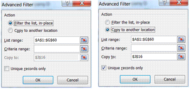
Figure 2
Use the choices under Action to either “Filter the list, in-place” (very much like what AutoFilter does) or to extract a Copy to another location of the selected data. I find the latter (i.e., copy to another location) to be the more useful feature since it leaves the original data untouched and all the rows remain visible. It also makes it possible to simultaneously view the results of different queries and to save the results of different queries for future review.
The List range field specifies the Excel range containing the source data. In our example it is Sheet1!A1:G60.
The Criteria range is optional. This might seem strange since shouldn’t a criteria be required to filter data? But, it turns out that leaving this out can be a powerful mechanism. Also, when specified, and unlike AutoFilter, the criteria are entered in a worksheet range. This, particularly when combined with copying the result to another location, allows one to “save” both the criteria and the corresponding result for future review. It also allows one to ask extremely sophisticated questions, since the content of the criteria range can be any Excel formula.
When the selected action is Copy to another location, the Copy to field allows one to specify where Excel should save the results. Use this field to specify which columns to include in the output.
Finally, the Unique records only checkbox indicates that the result should have no duplicate results, where duplicates are defined as having the same value in every output column.
As mentioned above, I am not a proponent of “Filter the list, in-place.” I have a strong preference for the alternative, ‘Copy to another location’ and it is how advanced filter is used in this document. However, if one does filter a data source in-place the way to remove the advanced filter is to click the Data tab | Sort & Filter group | Clear button.
There are two ways to specify the criteria for filtering or extracting data. This section addresses the one that is probably easier to understand. Duplicate the names of the columns of the source data in a single row in some empty range. Then, in the row under it, enter the different conditions. Conditions entered in the same row are ‘AND’ed together while conditions on separate rows are ‘OR’ed. This is possibly easier to understand with a few examples.
List all orders for NT Dried Plums
This requires specifying a single value for the Product column as shown in Figure 3. The dialog box also shows that the result will be copied to the range starting with J8.
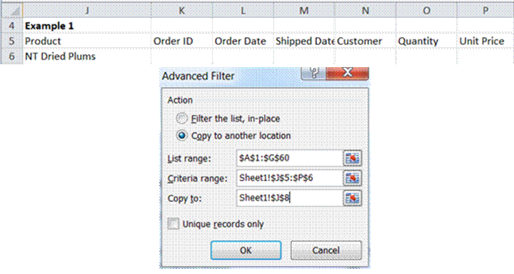
Figure 3
The result, shown in Figure 4, lists all the product orders that relate to NT Dried Plums.
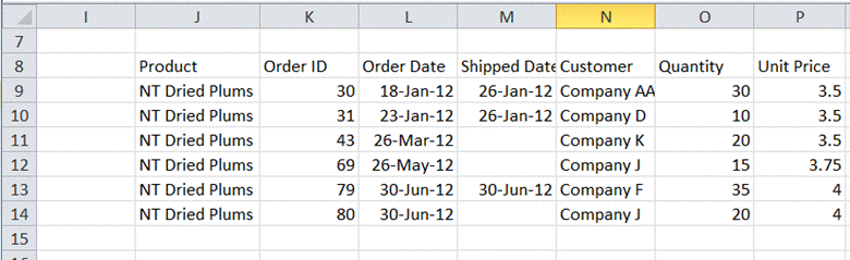
Figure 4
List all the orders for NT Dried Plums where the quantity is greater than 15.
The requirement translates to the criteria: Product=”NT Dried Plums” and Quantity >30. Since this is an AND condition, the two individual conditions will be on the same row. Also, it is enough to include only those column headers that contain a condition as in Figure 5.
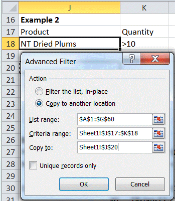
Figure 5
The result is in Figure 6.
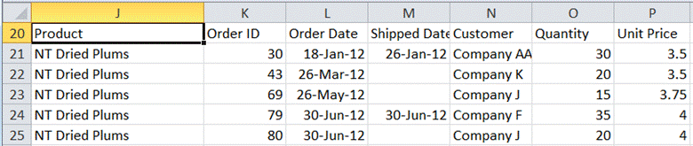
Figure 6
List all the orders for NT Dried Plums where the quantity is greater than 15 and less than or equal to 30.
In this case, the conditions are Product=”NT Dried Plums” and Quantity > 30 and Quantity <=30. Remember that ANDed conditions have to be on the same row and there are two conditions that involve Quantity! Luckily, Advanced Filter allows columns to be duplicated as in Figure 7.
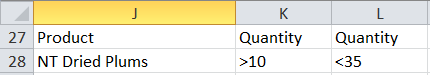
Figure 7
List the Order ID, Order Date, and Company Name for all orders for NT Dried Plums where the quantity is greater than 15 and less than or equal to 30.
This filter criteria is the same as in the previous example except that the output list should include only a subset of 3 specific columns. To accomplish this the Copy to field should specify only the headers of the desired columns as in Figure 8. If the header names do not match those of the source, Excel will raise an error.
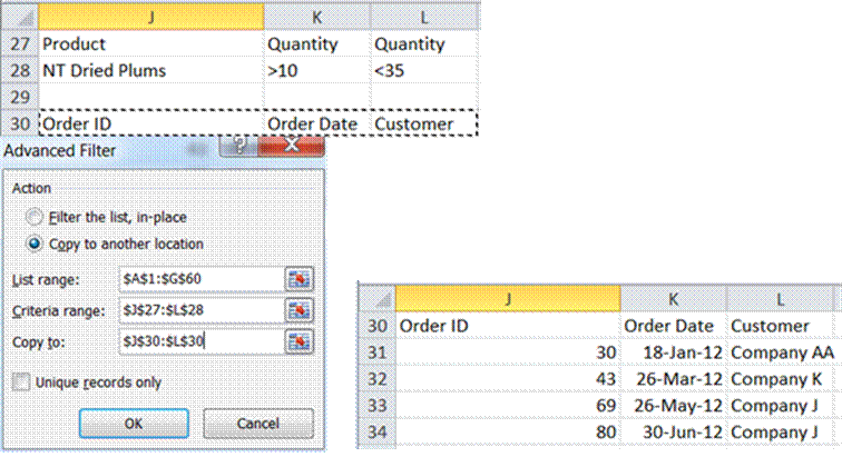
Figure 8
The last few examples have shown how to specify various elements of the Advanced Filter dialog box. Subsequent examples will focus on the conditions in the cells and may skip showing the contents of the Advanced Filter dialog box.
List all orders for either NT Dried Plums or NT Dried Pears.
Since the criteria involves an OR condition, the 2 values should be on different rows as in Figure 9.
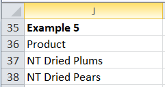
Figure 9
The result is in Figure 10.
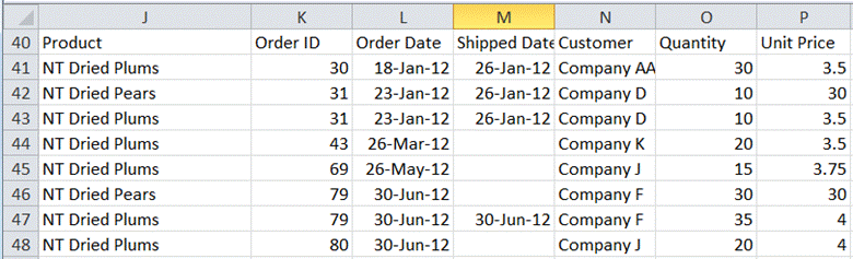
Figure 10
List the Product, Order ID, and Quantity for all orders for quantities greater than 10 and for either Dried Plums or Dried Pears.
Remember that AND conditions go in a single row and OR conditions go in separate rows. In this case, Excel will evaluate each row independentaly and then check the OR part. So, the correct way to write the logical requirement is (Quantity > 10 and Product=”NT Dried Plums”) or (Quantity > 10 and Product=”NT Dried Pears”) as in Figure 11
Figure 11
List all orders for NT Chocolate.
While previous searches also involved text fields what was not evident was that Excel actually matches values that start with the specified text. This becomes more obvious when the search is for “NT Chocolate,” which shows results for both NT Chocolate and NT Chocolate Biscuits Mix.
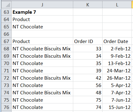
Figure 12
The way to search for an exact match is to enter the search string as a formula as shown in Figure 13, which shows the formula entered in J80.
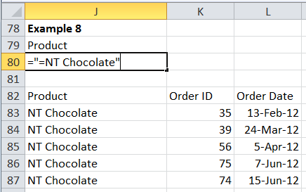
Figure 13
For all tea related products, list the product, the order id and the order date.
Tea related products are defined as having “tea” somewhere in the product name. Advanced Filter works with wildcard characters such as * and ?. To search for any occurrence of tea in the name of a product, use *tea*. [As in other context and other languages, the ? character allows a single character to be anything.]
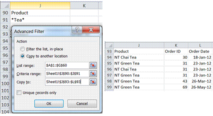
Figure 14
List the product, the order id and the order date for all products with names like t-any character-a.
The required condition includes a wildcard pattern, i.e., Product=*t?a*. The result includes, in additio to the various tea products, NT Almonds, in which the T-space-A combination satisfies the t?a pattern.
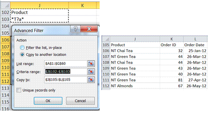
Figure 15
List all orders placed since June 1, 2012.
This is similar to the earlier conditions and it involves simply typing in the characters >6/1/2012. Excel will correctly interpret the content of the cell as a date (see Figure 16).
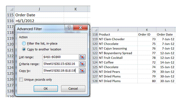
Figure 16
List all product orders for May 2012.
This is also similar to the previous example of 2 conditions on the quantity ordered (Example 3). Simply enter the conditions in the 2 cells as shown in Figure 17.
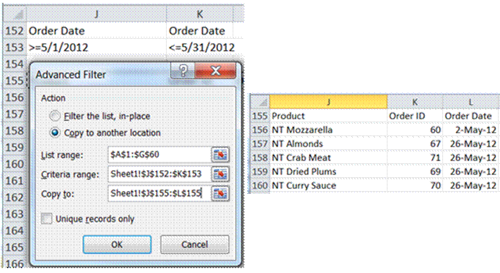
Figure 17
List all products that remain unshipped. Ensure that the output is verifiable.
An unshipped product will have an empty Shipped Date. Adapt the earlier suggestion for finding an exact match (Example 11) except this time specify nothing in the search expression as in Figure 18. Also, to ensure a verifiable output, include the Shipped Date column. Obviously, it should contain only empty cells.
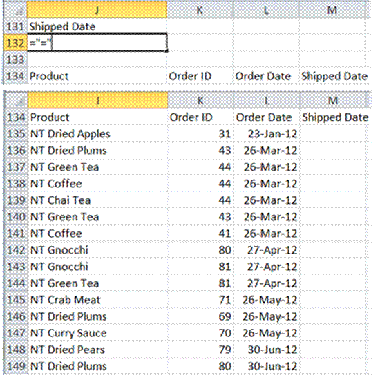
Figure 18
As versatile as the filter specification using the column name method is, there are fundamental restrictions on what one can do. The major reason for these restrictions is that each condition is limited to a specific column in each row. On the other hand, with the use of Excel formulas and functions it becomes possible to
· combine the data in different columns using, say, arithmetic operators,
· base the criteria on values across rows, and
· use a statistic (such as “top 10”) to compare a particular different rows.
The way to enter a formula as the filter criteria is similar to and yet somewhat different from the above examples. The important items to remember are:
1. In the criteria range the row containing the column headers must be blank.
2. Relative cell references to the data source must refer to the 1st data row in the source range.
3. The formula must yield a TRUE or FALSE result. That is how Excel decides whether to include a particular row in the result or not.
List all products that remain unshipped. Ensure that the output is verifiable.
This is the same as Example 12 but now instead of a “trick” to specify an empty cell, the formula is straightforward and easy to understand (Figure 19). As mentioned earlier, the criteria range must have a blank first row and the formula must refer to the 1st row with data.
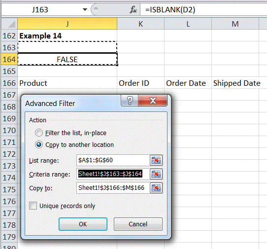
Figure 19
The result (Figure 20) is identical to that in Example 13.
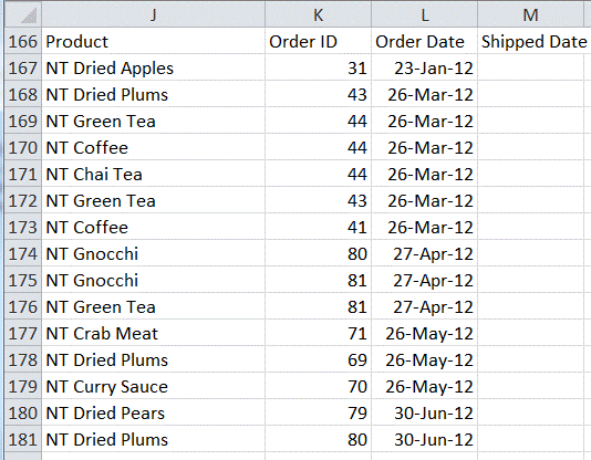
Figure 20
List all product orders that shipped more than 7 days after the order was place.
The condition requires checking if the difference between the product order date and shipped date is more than 7 days. [This specifically excludes unshipped orders.] Figure 21 shows both the criteria and the result.
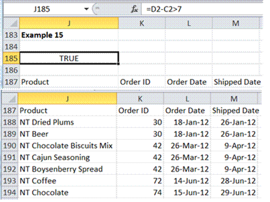
Figure 21
List all product orders that remain unshipped or were shipped more than 7 days after the order was placed.
This essentially is Example 14 combined with Example 15. The formula is shown in Figure 22.
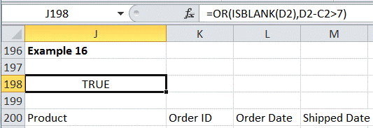
Figure 22
As of July 6, 2012, list all product orders that were ordered more than 7 days ago and remain unshipped.
This is similar to the previous example except that it involves an ‘and’ condition as well as a specific date in the formula (rather than comparing two dates that are already in the table). The formula and the associated result are in Figure 23. As should be expected the result should match Example 14 with the exception of the last 2 orders (order 79 and order 80), which were placed on June 30, 2012, i.e., 6 days before July 6, 2012.
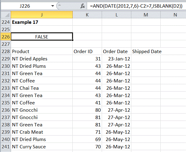
Figure 23
List all product orders that generated revenues in excess of 2,000.
This requires calculating the revenue from the existing columns. The revenue is the quantity (column F) multiplied by the unit price (column G), which makes the problem similar to Example 15 (which required calculating the difference between two columns). The criteria and the result are in Figure 24.
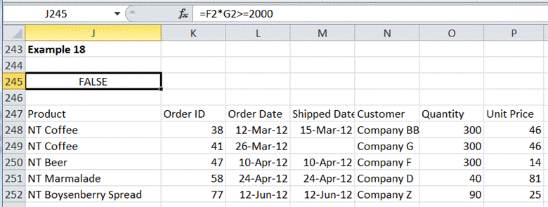
Figure 24
List all product orders where the entire order generated revenues in excess of 2,000.
This is similar to the previous example except that now the decision is based on the entire order. An order that includes multiple products will have one row for each product in the source range. Consequently, the filter criteria must sum the revenue for each product in the order corresponding the each row. In the formula below, the first argument of the SUMPRODUCT is --($B$2:$B$60=B2). The part in parenthesis generates a list of 59 TRUE or FALSE values, one for each row in the source data, based on whether the row is part of the current order or not. The double minus signs convert the TRUE/FALSE values in 1/0 values. The other arguments to the SUMPRODUCT include the quantity and the unit price. Consequently, Excel will SUM the PRODUCT of the 1s or 0s with the quantity and the unit price. This will yield the total revenue for the current order.
As one might expect, it includes all of the results from the previous example and also a few more. None of the individual products in Order 46 met the 2,000 threshold but as a complete order it exceeds 2,000 in revenue. One of the products in Order 58 was included in the previous result and as a result the entire order exceeds the 2,000 threshold. Consequently, the other smaller product order in Order 58 is now included in the result. For the criteria and the result see Figure 25.
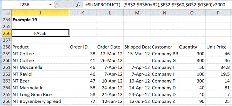
Figure 25
List all product orders where the quantity ordered is more than 50% greater than the average quantity.
In this example, the comparison will be between each row of data and a statistical measure applied to the entire data set. What is required is to test whether the quantity is more than 1.5 * average quantity ordered per product. This translates to the formula and result in Figure 26.
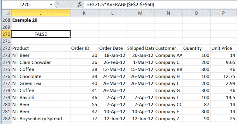
Figure 26
Array formulas, for those who know about them, represent a powerful computation capability within Excel. Unfortunately, the Advanced Filter criteria range cannot contain such a formula. If it does, Excel will return no results. Consequently, it becomes necessary to find a workaround, when possible, to the use of an array formula in a filter criteria formula.
List all product orders where the revenue is more than 50% greater than the average revenue.
This looks very much like Example 20 but it requires the use of a calculated field. The most obvious way might be the formula =(F2*G2)>1.5*AVERAGE($F$2:$F$60*$G$2:$G$60). This will yield a #VALUE! error since it must be entered as an array formula.
After than is done, and Advanced Filter is given this criteria range, the result will be no rows in the output.
An alternative formulation for this array formula is the non-array formula =(F2*G2)>1.5*SUMPRODUCT($F$2:$F$60*$G$2:$G$60)/COUNT($G$2:$G$60). With this criteria Excel returns the correct result for Advanced Filter as in Figure 27.
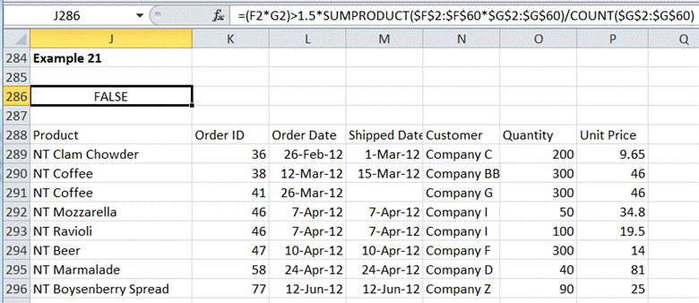
Figure 27
Obviously, not every array formula has an equivalent non-array formula and in those cases Advanced Filter will not provide the desired functionality.
The one element of the Advanced Filter dialog box that has remained unused has been the Unique records only checkbox. Select it to ensure that the result contains only unique records, where uniqueness means that no 2 rows have the same value in all the output columns.
This enables a set of useful results that identify unique values in various columns in the source data. For example, a list of every product that has been ordered at least once or a list of orders and their order dates.
It is also possible to specify a criteria together with the unique records only option to get concise results that satisfy the desired condition.
Provide a unique list of products that had at least one sale.
This is probably the easiest way to create a list of unique items in any column. When the Advanced Filter output range specifies a single column header, Excel will create a unique list of all the items in that column. This is an excellent example of the benefit of leaving empty the filter criteria field (see Figure 28).
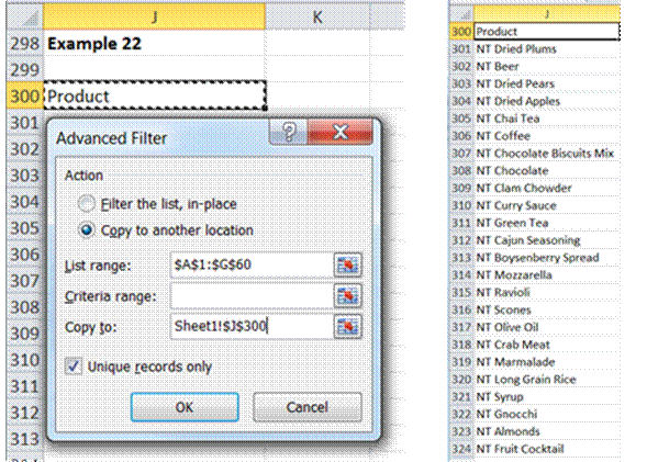
Figure 28
Create a unique list of dates when orders were placed and the corresponding orders.
The ability to create a unique list extends to multiple columns. When more than 1 column is involved, uniqueness is defined as having a different value when all columns are taken into account. Consequently, the same value may appear multiple times in the one column (as the date in Figure 29) but the values across all the columns together will be unique.
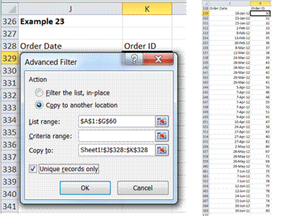
Figure 29
List all customers affected by unshipped orders placed earlier than 7 days prior to July 6, 2012.
This is similar to Example 17 except that the result should be a unique list of affected customers as in Figure 30.
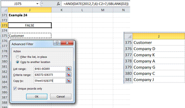
Figure 30
Some of the formulas used as filter criteria referred to the entire column of data using absolute references (e.g., $G$2:$G$60). Obviously, these formulas would require revision if the source data range were to expand.
There are two ways to create a reference that dynamically adjusts itself. One is the use an Excel table. The other is to use a named formula that creates a dynamic range reference. Given how flexible Excel tables are, we will look at only that way of creating a dynamic reference. To convert the same data set into an Excel table, select any cell in the data source, then select the Insert tab | Tables group | Table button. In the example workbook, the TableFilter worksheet contains the source in table form. The first few rows in the table look like Figure 31.
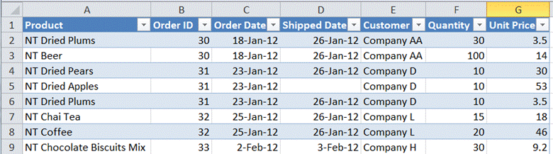
Figure 31
List all product orders where the entire order generated revenues in excess of 2,000.
This is the same problem as Example 19. As always, it’s easiest to create the formula using the mouse to click, point, and drag as appropriate. Selecting all the data in a column will result in Excel converting the range reference into a table reference. Note the difference in the dialog box source data field as well as in the formula in the criteria cell (Figure 32). The result is identical to that in Example 19.
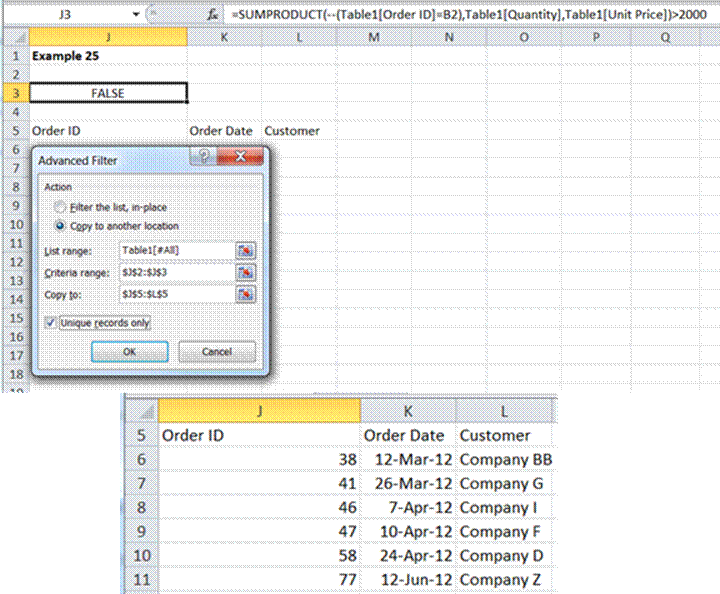
Figure 32
When the criteria and the result are in a different worksheet than the source range, it is important to initiate the Advanced Filter dialog box with the destination sheet as the active sheet. This is because Excel will insist on copying the results to the active sheet. So, with the table in the worksheet TableFilter and the destination sheet as Sheet2, select Sheet2, create the necessary criteria and output headers and then click the Advanced Filter button. Also, it will be easiest if the active cell is an empty region. Otherwise, Excel will attempt to guess the locations of various ranges and, as a result, it might raise an error. Figure 33 is an example of an Advanced Filter dialog box with Sheet2 as the active sheet.
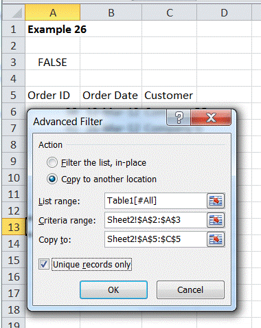
Figure 33
Working with the source list in another workbook is similar. Start with the destination worksheet in the destination workbook. The rest of the mechanics of creating the criteria formula and the references in the dialog box are the same. Obviously, the references are longer because, now, they also have to include the workbook name as in Figure 34.
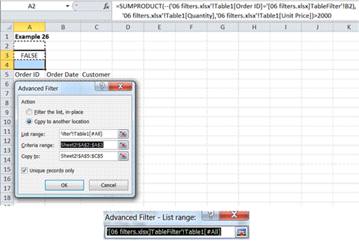
Figure 34
One final note on working with another workbook: Even when copying the data to another location, the source workbook must be open for Advanced Filter to work.
This document provides what is hopefully a comprehensive review of the Advanced Filter capability in Excel 2010 and Excel 2007.
Excel 2010, Excel 2007, data analysis, advanced filter; advance filtering; custom filter; filter advanced; advanced filter criteria; remove advanced filter; advanced data filter; advanced sort & filter;

