![]() 2010 (32-bit and 64-bit)
2010 (32-bit and 64-bit)
![]() 2007
2007
![]() 2003
2003
Dashboards are a popular and convenient way to visually examine data. However, if a chart displays something that warrants further investigation, there is no way to do so from the chart itself. To "drill down" to the underlying data one must go back to the originaldata and analyze the relevant subset. Alternatively, one can delegate the task to a subordinate and have her/him do the work.
The TM PivotChart Drilldown feature of the add-in supports a single-click drill down capability. Click on a PivotChart's data point and the add-in will show the details of the underlying data in the same chart. Each click drills down to the next more detailed level and a click on the lowest (most detailed) level returns the chart to the summary view.
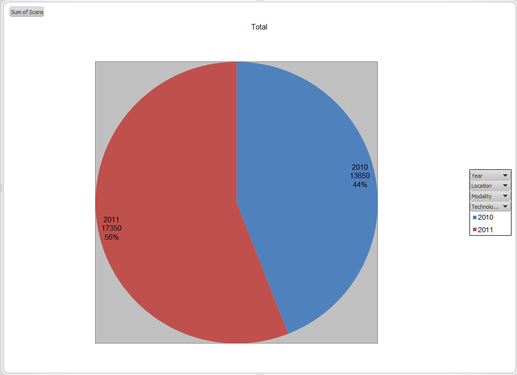
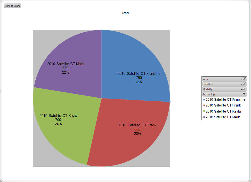
The example below shows a PivotChart reporting on the number of annual scans of different types performed by each technologist at a radiology department with two locations (the 2011 data are projected scan volume). The PivotTable corresponding to the PivotChart has 4 row fields (Year, Location, Modality, and Technologist) and 1 data field (Sum of Scan).
Create a PivotTable and a PivotChart (on its own sheet) with 4 row fields (Year, Location, Modality, and Technologist) and 1 data field (Sum of Scan). This example uses a pie chart but the software works with any PivotChart.
Then, with the TM PivotChart Drilldown feature
enabled, the "highest level" PivotChart will show a summary for the 2 years, 2010
and 2011.
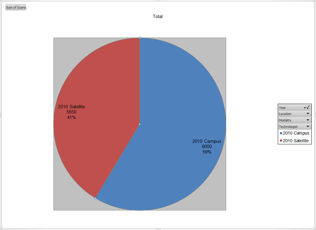
Click on the 2010 point to see the underlying data for the two
locations where services were available in 2010: Campus and Satellite.
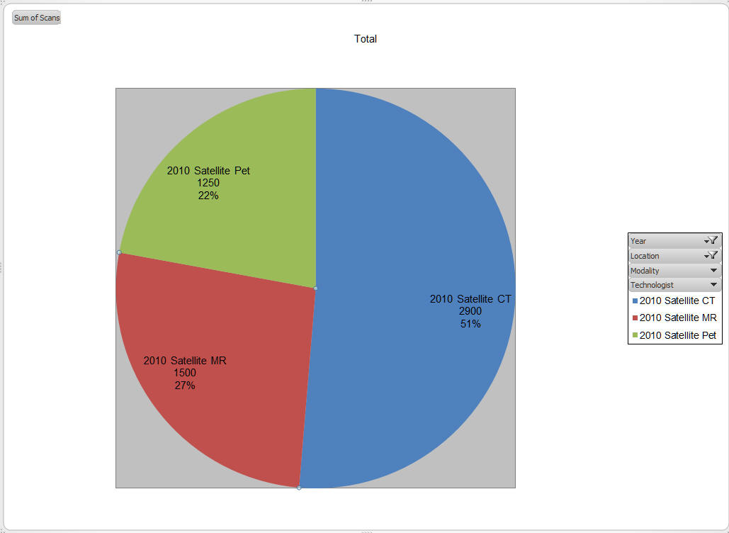
Click on the Satellite data point to see the data for the 3
modalities supported at that site in 2010: MRI, CT, and PET scans.
A click on the CT data point shows the number of CT scans by each technologist at the Satellite location for the year 2010. This is the
most detailed level of data in the PivotChart (and the corresponding
PivotTable).
Finally, a click on any of the data points returns the chart to the
highest level, i.e., the year-by-year summary.
Download either the self installing executable or the zip file. Use of the self-installer will also enable an uninstall feature. Alternatively, unzip the contents of the zip file into a convenient folder, though Excel's Add-Ins folder is strongly recommended.
For more see Common Installation Instructions. In the last step, to load the add-in, select the checkbox next to TM PivotChart.
In Excel 2007 and 2010, enable the drilldown capability by clicking the TM tab | Pivot group | PivotChart Drill-down button.
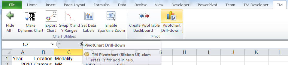
Another way to reach the same dialog box is to select a PivotChart and then select from the PivotTable Tools contextual tabs: TM tab | Pivot group | PivotChart Drill-down button.
In Excel 2003 (or earlier), select TM | PivotChart Drill-down > Enable.
This add-in has the following prerequisites:
The PivotChart must be in its own chartsheet.
The corresponding PivotTable must have no column fields and only 1 data field.
Now, click on any chartsheet that contains a PivotChart and the add-in will modify the chart to show a "high level" summary.
To turn off the drill-down capability click the PivotChart Drill-down button again.
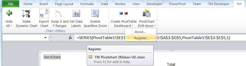
The add-in comes with a trial period, after which continued use requires a registration key. Once you get the registration key, to enter it select the PivotChart Drill-down's dropdown menu | Register...
Contact the author through his website at www.tushar-mehta.com

