One of the frequent requirements in developing an Excel worksheet is validating that the user actually does enter certain mandatory information. There are some who believe that it requires VBA to enforce this requirement. However, one can essentially do the same without any programming. This tip shows one possible way.
The basic idea is to incorporate a test for the mandatory data into one (or more) key formulas. If the required data are not entered, the formula returns an obviously wrong result, or better yet, an error message of sorts. If the formula returns a wrong result it must be so obviously wrong that no reasonable person would use that result for any real decision.
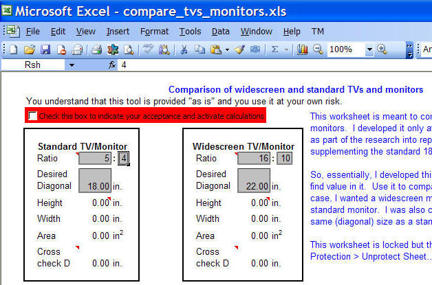
The easiest way, as often, is to illustrate the idea with an example. In creating the worksheet to compare TVs and computer monitors of different sizes, as an after-thought I decided to include a warning that the worksheet was available on an "as-is" basis. Further, I wanted the user to check a checkbox to indicate acceptance of the "as is" status.
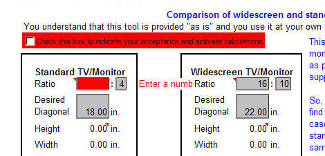
Since this warning was added "after the fact," including a error message would have required a bit of a redesign of the worksheet. Instead, I chose to return a result that would be obviously wrong -- a screen height of zero! Figure 1 shows a portion of the worksheet. All the calculations would return zeros until the user selects the checkbox 'Check this box to indicate your acceptance.'
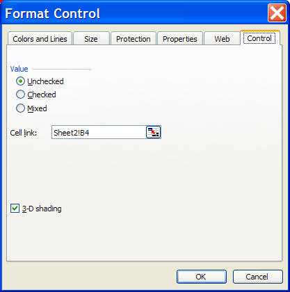
The solution requires linking the checkbox
to a worksheet cell, which will contain either a TRUE or a FALSE
(or a blank value if the checkbox has never been checked).
The formula for the 'Height' calculation incorporates this
TRUE/FALSE cell in a simple IF formula:
=IF({cell-with-Boolean-value},{correct formula},0).There's one more item to
think about before implementing this idea. Eventually,
this worksheet will be locked. But, the cell linked to the
checkbox must be unlocked. So, if the linked cell was in
this worksheet the user could accidentally, or intentionally,
change its value. Work around this problem by using a cell
in a new worksheet (or using an already present but otherwise
unused worksheet). Hide but do not protect this new
worksheet.
OK, so, let's designate a cell, say B4 as the linked cell.
Next, modify the formula for the height calculation to include this cell in the IF statement indicated above: =IF(Sheet2!B4,Rsh/SQRT(Rsw^2+Rsh^2)*Ds,-1)
That's it! Until the user selects the checkbox, the worksheet returns height and width values that are clearly and obviously wrong.
The above incorporates one mandatory item into the calculations such that if that item is missing none of the calculations work. But, can we include additional items and different types of validations? For example, in the above example, can we extend the validation requirements? After all, each of the four cells that specify the two aspect ratios should contain a number.
One easy way to do this is to create a single cell that contains TRUE if all the data validation criteria are met. On Sheet2 (unhide it if necessary), use cell B6 for that purpose. It will have the formula =AND(B4,ISNUMBER(Rsw),ISNUMBER(Rsh),ISNUMBER(Rww),ISNUMBER(Rwh))
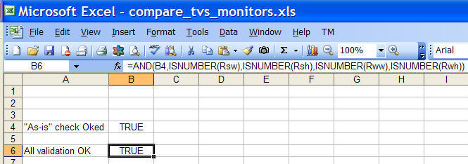
Finally, we modify the formulas on Sheet1 that referenced Sheet2!B4 to refer to Sheet2!B6 and we are all set.
Why not use Excel's native data validation capability? While it is a very powerful capability, there are two problems with it. First, the validation is triggered only when the user tries to enter something in that cell. So, if the user never edits the cell contents, they are never validated. Second, if the user pastes a value into the cell, all the validation is typically destroyed! By using our own validation, we avoid both of those problems.
Of course, we should be sufficiently user-friendly to help identify the error. We will do that with changes to Sheet1. Again, remember all this validation is after-the-fact and consequently, we need to make our error messages fit into the existing layout.
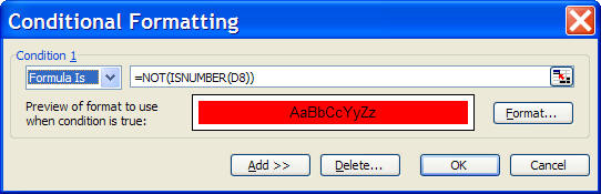
In cell H8 (on Sheet1) enter the formula =IF(NOT(AND(ISNUMBER(Rsw),ISNUMBER(Rsh),ISNUMBER(Rww),ISNUMBER(Rwh))),"Enter a number!","") Format this cell to have a red font. Next, select D8 and add a conditional format as below:
Once done, copy D8 to F8, K8, and M8. Remember to reset the values in those cells. Now, if any of the aspect ratio cells do not contain a number, the worksheet will look like: