Excel's RANK function ranks a number within a given range of numbers. The syntax is
RANK(number,ref,order)
Number is the number whose rank you want to find.
Ref is an array of, or a reference to, a list of numbers. Nonnumeric values in ref are ignored.
Order is a number specifying how to rank number.
If order is 0 (zero) or omitted, Microsoft Excel ranks number as
if ref were a list sorted in descending order.
If order is any nonzero value, Microsoft Excel ranks number
as if ref were a list sorted in ascending order
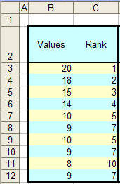
As intended, RANK gives the same rank to duplicates and resumes ranking for subsequent numbers after leaving a gap. For example, consider a scenario where numbers are ranked in descending order. If the number 10 appears twice in a list with a rank of 5, the next number, say 9, would have a rank of 7. Similarly, since 9 appears 3 times, the next number, 8, has a rank of 10. The formula in C3: =RANK(B3,$B$3:$B$12) Copy C3 as far down as there are data in column B.
There are instances when this result is not acceptable. This page looks at three ways to modify the result of Excel's RANK function.
To simplify the formulas, create two names (Insert | Name > Define...)
The first refers to the original data range, the other to the adjacent cells containing the unmodified RANK formula.
DataRng =Sheet1!$B$3:$B$12
RankRng =OFFSET(DataRng,0,1)
| Adjust a tie so that it reports the
"middle" value. In the first cell containing the rank, enter the formula =RANK(B3,DataRng)+(COUNTIF(DataRng,B3)-1)/2 Copy as far down as there are data in DataRng Note that the Excel help file recommends the more complex correction factor =(COUNT(ref) + 1 � RANK(number, ref, 0) � RANK(number, ref, 1))/2
|
 |
| Use a tie breaker to create a unique
rank
In the first cell containing a rank, enter the formula =RANK(B3,DataRng)+COUNTIF($B$3:B3,B3)-1 Copy as far down as there are data in DataRng.
|
 |
| A variant of the tie break that
assigns ranks in reverse order In the first cell containing a rank, enter the formula =RANK(B3,DataRng)+COUNTIF(DataRng,B3)-COUNTIF($B$3:B3,B3) Copy as far down as there are data in DataRng. |
 |
| Retain duplicate values but create
continuous ranks, i.e., no breaks in the rank. In the first cell containing a rank, enter the array formula1 =SUM(1/(IF(RankRng<C3,COUNTIF(RankRng,RankRng),9.999999999E+307)))+1 Copy as far down as there are data in DataRng.
Accomplish the same with the new IFERROR function introduced with Excel 2007. In the first cell containing a rank, enter the array formula1 =SUM(IFERROR(1/COUNTIF(RankRng,IF(RankRng<C3,RankRng)),0))+1 Copy as far down as there are data in DataRng.
1 To enter an array formula complete data entry with the CTRL+SHIFT+ENTER combination and *not* with the ENTER or TAB key. |
 |
References: See Chip Pearson's http://www.cpearson.com/excel/rank.htm

