Step 1: Create a chart

The example below uses a simple XY scatter chart.

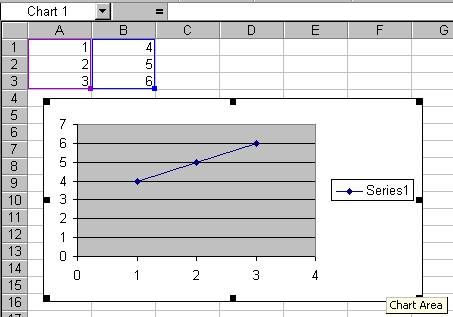
Figure 1

Step 2:  Add a title

Use chart options to add a title.  This is shown in Figure 2 and Figure 3.  Note that if you use the chart wizard to create a chart, the title can be added in one of the wizard's dialog boxes.

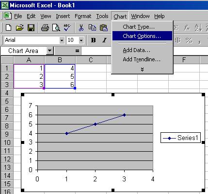
Figure 2

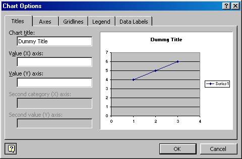
Figure 3

Step 3: Change the title to a dynamic title.

Select the title box as shown in Figure 4. 

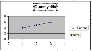
Figure 4

Type the '=' key (without the quotes) and click on the cell that will contain the formula for the title.  In the example, it is cell D1 (see Figure 5).

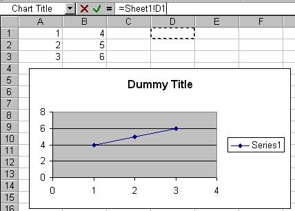
Figure 5

Step 4:  Enter the required formula in cell D1.

In this example, the formula is shown in Figure 6.

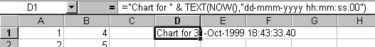
Figure 6

Step 5: Enjoy the end product

The final result is shown in Figure 7.

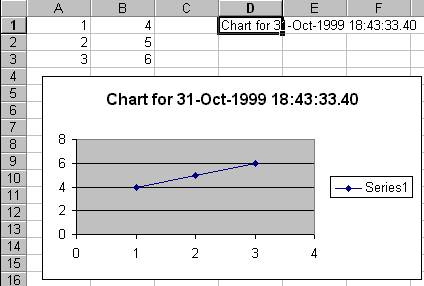
Figure 7